Excel Tips

Nonprofit Technology Collaboration

Last Updated: 11/8/2013 Excel Tips Page 1 of 15

Excel Tips

Contents

Cell Referencing ................................................................................................................... 2

Recovering Unsaved Workbooks ......................................................................................... 6

Identifying Duplicate Values ................................................................................................ 8

Removing Duplicate Values ............................................................................................... 10

Switching Rows and Columns ............................................................................................ 12

Separating Columns ........................................................................................................... 14

Nonprofit Technology Collaboration

Last Updated: 11/8/2013 Excel Tips Page 2 of 15

Cell Referencing

All data in Excel is stored in cells of worksheets. Worksheets are similar in concept to tables with

columns and rows. A cell is the point where a column and row meet. When referencing data in a “cell”

of a worksheet, you use a Cell Reference. A cell reference consists of a combination of the column letter

and row number that intersect to form the cell.

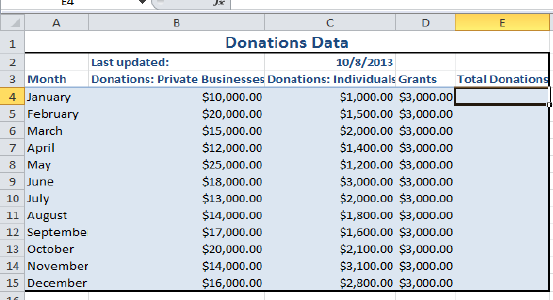
In Excel, there are two main types of cell references: relative cell references and absolute cell

references. Relative cell references identify the location of a cell by its column letter and row number

combination, with no added symbols. In the screenshot below, the currently selected cell would be

referenced as E4, which is a relative cell reference. Relative cell references are the default method of

referencing cells in Excel.

Absolute cell references also reference cells by a combination of column letter and row number, but

these references include a dollar symbol ($) before the column letter and before the row number. In

the screenshot above, the currently-selected cell would be referenced as $E$4 if I wanted to use an

absolute cell reference.

Using Relative vs. Absolute Cell Referencing

Cell references are frequently used in Excel formulas and functions. When relative cell references are

used in formulas or functions, if the formula/function is copied from the original cell to other cells, the

relative cell references will automatically change to reflect the new location of the formula/function.

When absolute cell references are used in formulas or functions, then if the formula/function is copied

from the original cell to other cells, the absolute cell references will not change—they will retain the

original cell reference. Note that a combination of relative and absolute references can be used in

formulas and functions.

Nonprofit Technology Collaboration

Last Updated: 11/8/2013 Excel Tips Page 3 of 15

Relative Cell Referencing Example

In this example, we have a set of data for all the donations a company has received from private donors,

individual donors, and grants. We want to calculate the total donations each month and will use relative

referencing to do this.

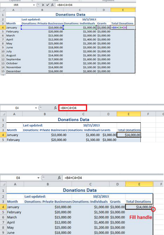
1. In this example we want to total the donations from the private businesses, individuals, and

grants. To do this, we will enter the formula shown below in cell E4 to calculate the desired

value. Note that the references to B4, C4, and D4 are all relative cell references.

2. Click enter and the total donations for the month of January will be calculated and displayed in

cell E4. Notice that the formula we just entered can be viewed in the formula bar.

3. Now we want to copy this same formula down the column so that the remaining month’s totals

can be similarly calculated. To do so, locate the fill handle in the lower right corner of cell E4.

Nonprofit Technology Collaboration

Last Updated: 11/8/2013 Excel Tips Page 4 of 15

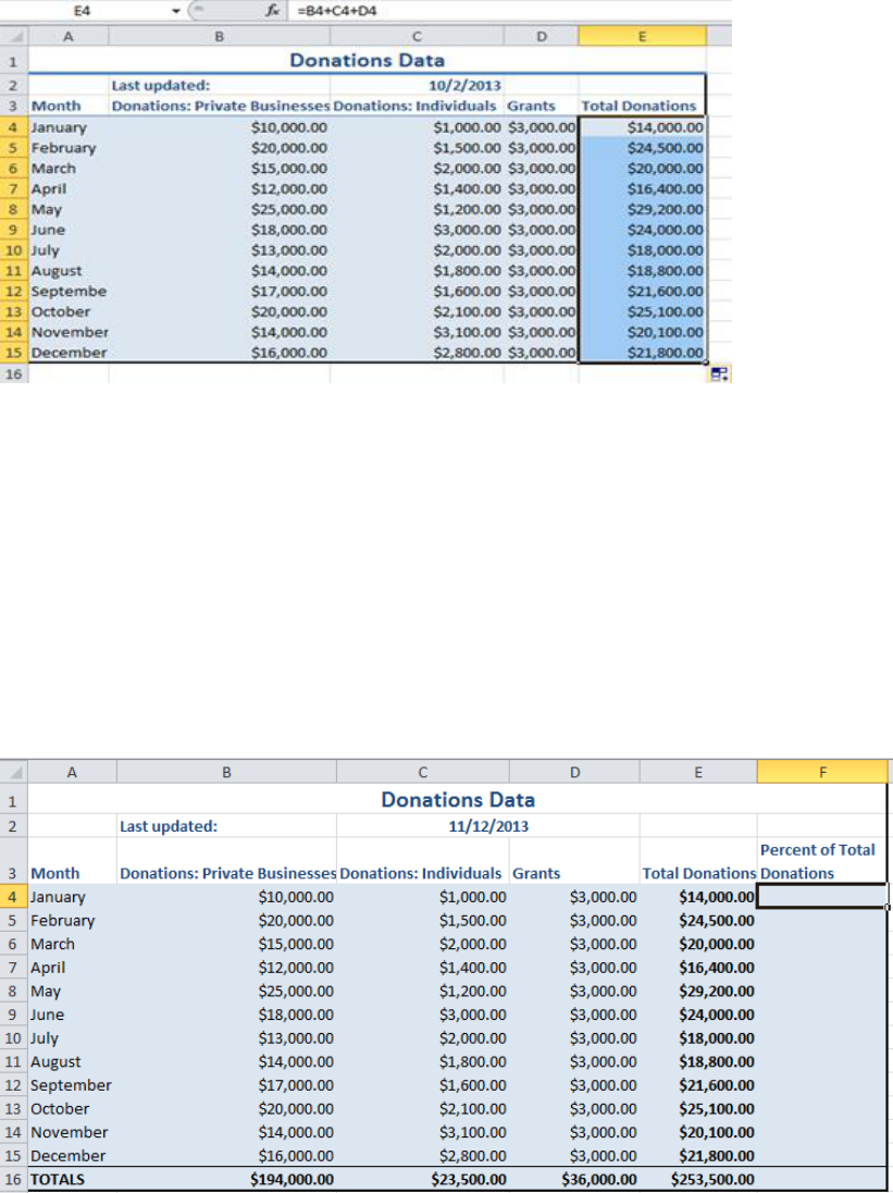
4. Now click and drag the fill handle over the cells you wish to copy the formulas into. Once you

release your mouse, the cells you wished to “fill” will contain a copy of the formula using the

relative cell references. Notice how the cell references change to reflect the current row. This is

a result of using relative cell references.

Absolute Cell Referencing Example

Absolute referencing is when you do not want a cell reference to change and you want the specific

value in that cell to stay fixed. Unlike in a relative reference, when you use the fill handle or copy/paste

a formula that uses absolute references, the absolute cell references for that formula will not change.

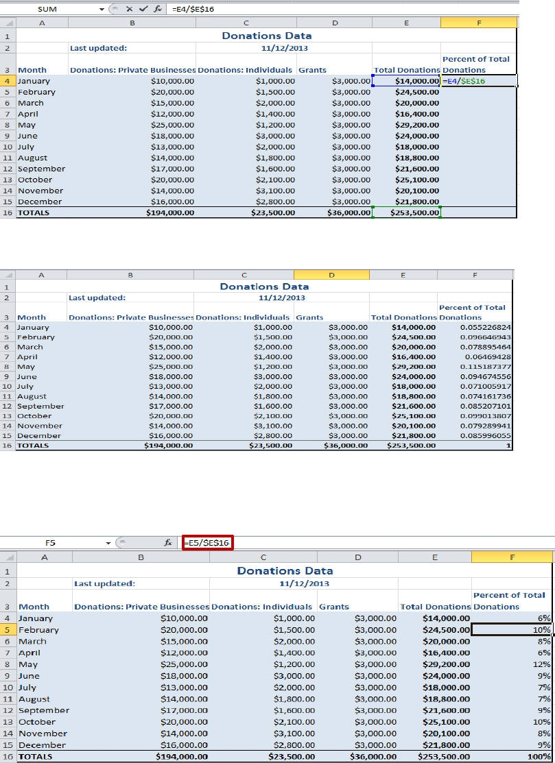
For this example, we want to calculate the percent of total donations for each month and store these

percentages in column F. In order to do this we will have to create a formula that divides our total

monthly donations by our total donations for the year. The total donations for the year is currently

stored in cell E16, which shows the total to be $253,500.00.

Nonprofit Technology Collaboration

Last Updated: 11/8/2013 Excel Tips Page 5 of 15

1. In our first month, January, we will enter a formula in F4 that divides January’s total donations

(stored in cell E4) by our total donations for the year (stored in cell E16). However, when we

subsequently copy this formula down the column to calculate the percentages for the other

months, we want the reference to the total donations for the year (in cell E16) to remain the

same. Therefore an absolute cell reference is used for the total donations for the year: $E$16.

2. Again, use the fill handle to repeat the formula for the next months. (See steps 3 and 4 in

previous example for how to use the fill handle.)

3. Notice how the reference for cell E16 has not been changed. This is a result of using an

absolute reference. Also note that we clicked the “%” button on the Excel ribbon in order to

format all the percentages to include the “%” sign.

Nonprofit Technology Collaboration

Last Updated: 11/8/2013 Excel Tips Page 6 of 15

Recovering Unsaved Workbooks

It’s painful when you accidentally close a workbook without saving it, then regret it later. To avoid this

scenario, remember to save your changes often. However, you can sometimes recover your work.

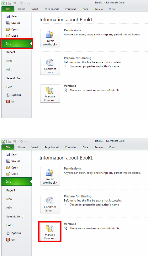
1. Click on the File button

2. Choose Info on the left side of the page.

3. Click the Manage Versions button.

Nonprofit Technology Collaboration

Last Updated: 11/8/2013 Excel Tips Page 7 of 15

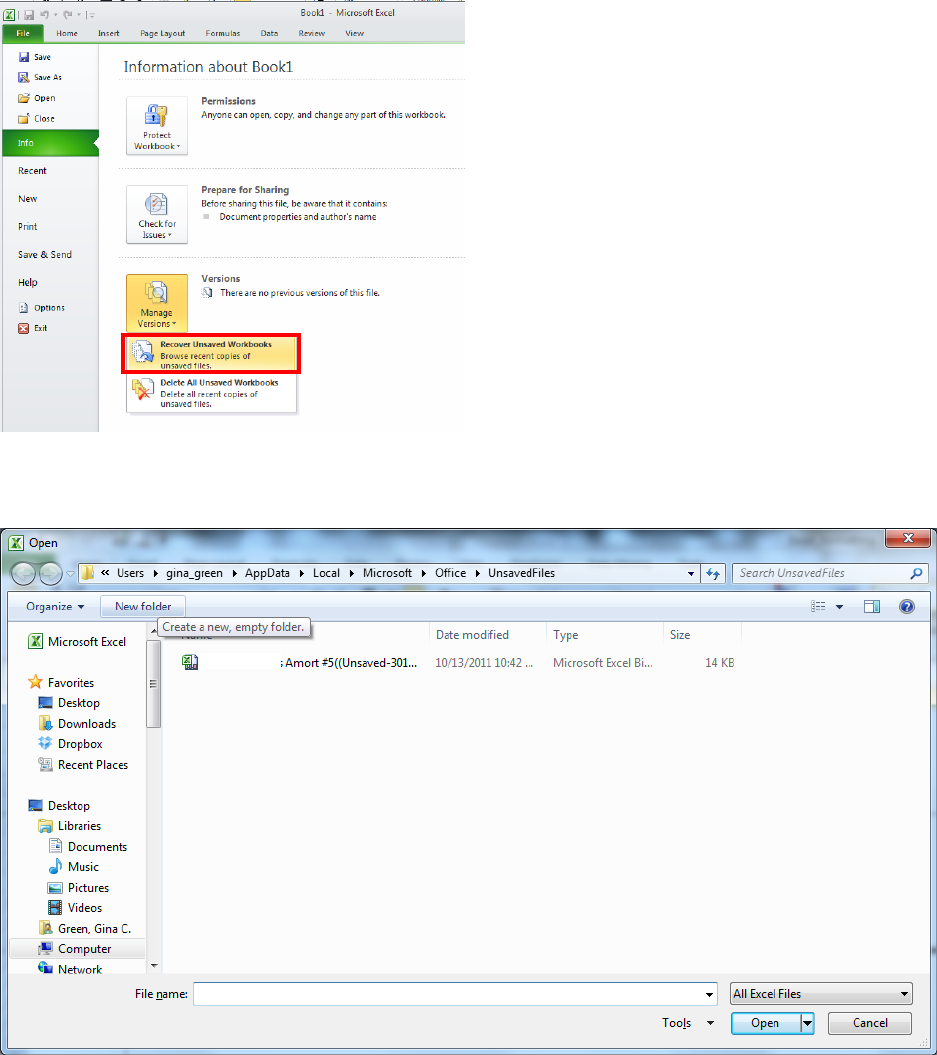
4. Choose Recover Unsaved Workbooks.

5. You’ll be presented with a list of workbooks with changes that were unsaved. Choose the

workbook you want to recover and click open. Then you will be able to save the workbook.

Nonprofit Technology Collaboration

Last Updated: 11/8/2013 Excel Tips Page 8 of 15

Identifying Duplicate Values

In worksheets with lots of data, you may have difficulty identifying duplicate values. Excel can search

data and highlight the duplicate values in a selected range.

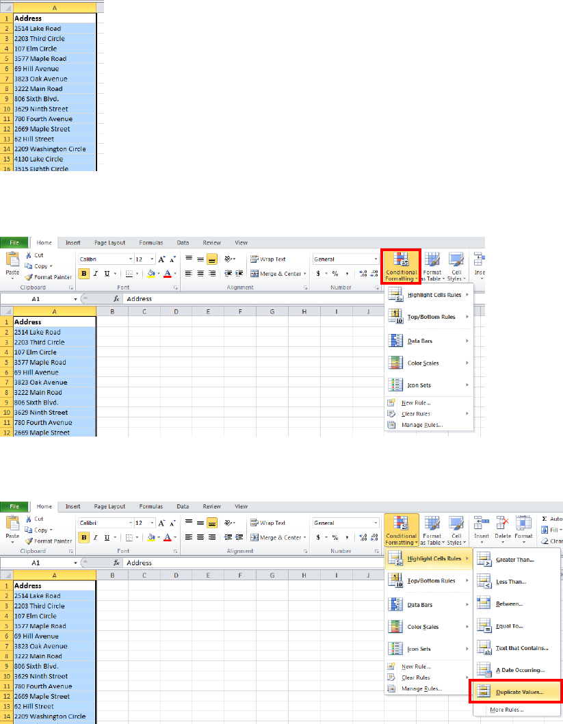
1. Select a range of values you want to search.

2. Go to the Home tab on the ribbon and Click Conditional formatting. This will display the

Conditional formatting menu.

3. From the Conditional Formatting menu, select Highlight Cell Rules. Then, choose Duplicate

Values.

Nonprofit Technology Collaboration

Last Updated: 11/8/2013 Excel Tips Page 9 of 15

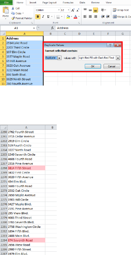
4. Choose the type of formatting you would like to apply to the duplicate cells in the Duplicate

Values dialogue box. This dialogue box allows you to see a live preview, or displays what will

happen to the cells as you click on the different options.

5. Click OK on the Duplicate Values dialogue box. All the duplicate values are now formatted

differently than other values.

Nonprofit Technology Collaboration

Last Updated: 11/8/2013 Excel Tips Page 10 of 15

Removing Duplicate Values

If you are using your Excel spreadsheet to organize data, you may want to identify duplicate values and

remove values that have already been repeated so your information will be as accurate as possible.

1. Select the range of cells that you want to check for duplicates. You can do this by clicking on the

letter or number corresponding to the column or row.

2. Go to the Data tab on the ribbon and click Remove Duplicates.

3. Make sure that the columns containing potential duplicates are selected in the Remove Duplicates

screen; If so press OK. If not, you have the option to unselect rows or columns.

Nonprofit Technology Collaboration

Last Updated: 11/8/2013 Excel Tips Page 11 of 15

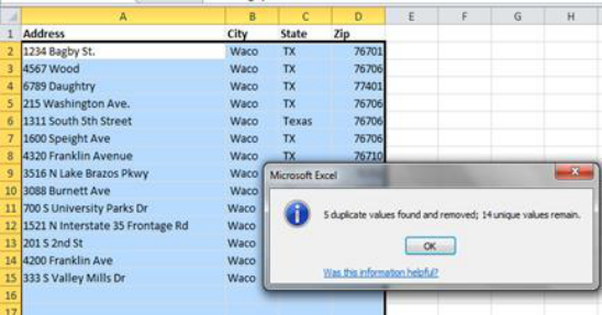
4. A message pops up telling you how many duplicates, if any, were removed and how many unique

values remain.

Nonprofit Technology Collaboration

Last Updated: 11/8/2013 Excel Tips Page 12 of 15

Switching Rows and Columns

Sometimes, you finish a worksheet and realize you want to re-organize the data. Excel allows you to

switch rows and columns easily.

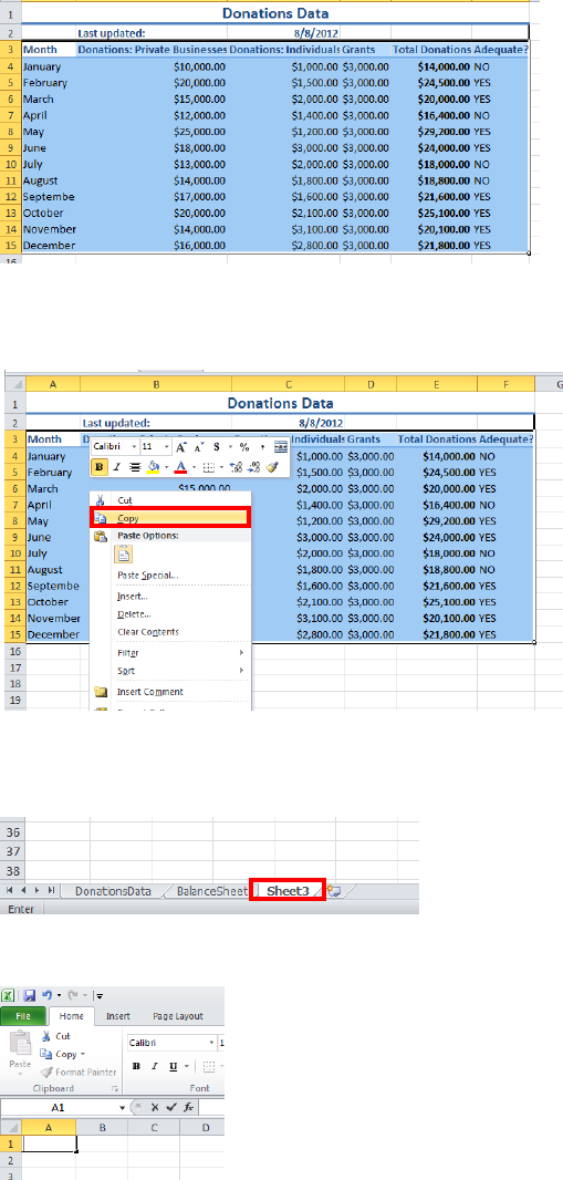
1. Select the range of cells that you want to switch the arrangement of rows and columns.

2. From the Edit menu, select Copy.

3. At the bottom of the page, click the tab for the worksheet you want the range to appear in.

4. On the worksheet, click the cell that you want the values to start in.

Nonprofit Technology Collaboration

Last Updated: 11/8/2013 Excel Tips Page 13 of 15

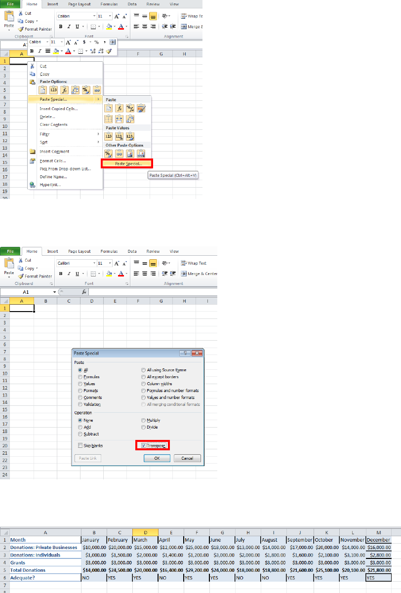
5. From the Edit menu, select Paste Special. The Paste Special dialogue box should appear.

6. Click the checkbox for Transpose in the Paste Special dialogue box.

7. Click OK. The data formerly presented down columns is now presented across rows and vice

versa.

Nonprofit Technology Collaboration

Last Updated: 11/8/2013 Excel Tips Page 14 of 15

Separating Columns

If you want to separate content that is currently in a single cell, (i.e. address, city, state, zip), you will

want to use the Convert Text to Column feature so that each characteristic will have its own cell. All of

the data that you want to be separated into different columns should either be separated by tabs,

semicolons, commas, or spaces.

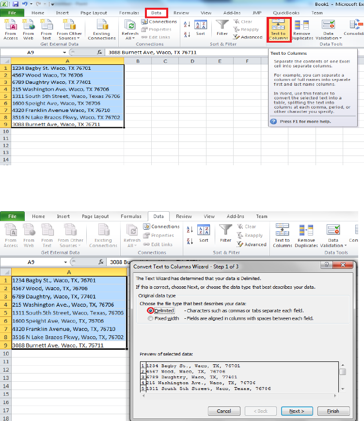
1. Assume you have a column of addresses that include the street address, town, state, and zip

code. You want to put each address component in separate columns on an Excel worksheet.

Highlight all of your data, then go to the Data ribbon and click the Texts to Column in the Data

Tools group.

2. On the first Convert Text to Columns Wizard screen, the Delimited file type should be selected.

Click Next to proceed.

Nonprofit Technology Collaboration

Last Updated: 11/8/2013 Excel Tips Page 15 of 15

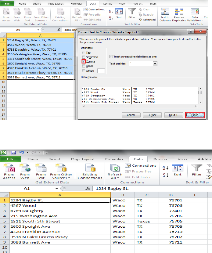
3. In this example, the address, city, state, and zip code are separated by commas. Deselect the

Tab delimiter and click the Comma delimiter. At the bottom of the Wizard screen, you can see a

preview of how your data will be separated. Click Finish to proceed.

4. All of your information will now be separated into individual cells.