
2/18/2020 MonteCarloMethods
localhost:8888/notebooks/GitCourseRepo/cs357-sp20/assets/demos/6-monte-carlo/MonteCarloMethods.ipynb#b)-Write-a-function-to-evaluate-the-probability-the-p
…
1/36
Randomness
What type of problems can we solve with the help of random numbers?
We can compute (potentially) complicated averages:
How much my stock/option portfolio is going to be worth?
What are my odds to win a certain competition?
Random Number Generators
Computers are deterministic - operations are reproducible
How do we get random numbers out of a deterministic machine?
In[1]:
Using the library numpy.random to generate random numbes:
In[2]:
If you want to generate a random integer number over a given range, you can use
np.random.randint(low,high)
that returns a random integer from low (inclusive) to high (exclusive).
In[3]:
Note that if you use the library random to accomplish the same thing:
random.randint(low,high)
the function returns a random integer from low (inclusive) to high (inclusive).
In[4]:
Generating many random numbers at one, using a numpy array:
Out[2]:
array([0.95478443, 0.00749089, 0.69214758, 0.82451778, 0.14715585,
0.91585328, 0.61205671, 0.65710847, 0.69876847, 0.32675238])
Out[3]:
3
Out[4]:
1
import numpy as np
import random
np.random.rand(10)
np.random.randint(1,10)
np.random.randint(1,10)
1
2
1
1
1

2/18/2020 MonteCarloMethods
localhost:8888/notebooks/GitCourseRepo/cs357-sp20/assets/demos/6-monte-carlo/MonteCarloMethods.ipynb#b)-Write-a-function-to-evaluate-the-probability-the-p
…
2/36
In[5]:
They all seem random correct? Let's try to fix something called seed using
np.random.seed(10)
What do you observe?
Let's see what this seed is...
Pseudo-random Numbers
Numbers and sequences appear random, but they are actually reproducible
Great for algorithm developing and debugging
How truly "random" are these numbers?
Linear congruential generator
Given the parameters , , and , where is the seed value, this algorithm will generate a
sequence of pseudo-random numbers:
In[6]:
In[7]:
In[8]:
for x in range(0, 20):
numbers = np.random.rand(6)
#print(numbers)
s = 3 # seed
a = 37 #10 # multiplier
c = 2 # increment
m = 19 # modulus
n = 60
x = np.zeros(n)
x[0] = s
for i in range(1,n):
x[i] = (a * x[i-1] + c) % m
import matplotlib.pyplot as plt
%matplotlib inline
1
2
3
1
2
3
4
1
2
3
4
5
1
2
2/18/2020 MonteCarloMethods
localhost:8888/notebooks/GitCourseRepo/cs357-sp20/assets/demos/6-monte-carlo/MonteCarloMethods.ipynb#b)-Write-a-function-to-evaluate-the-probability-the-p
…
3/36
In[9]:
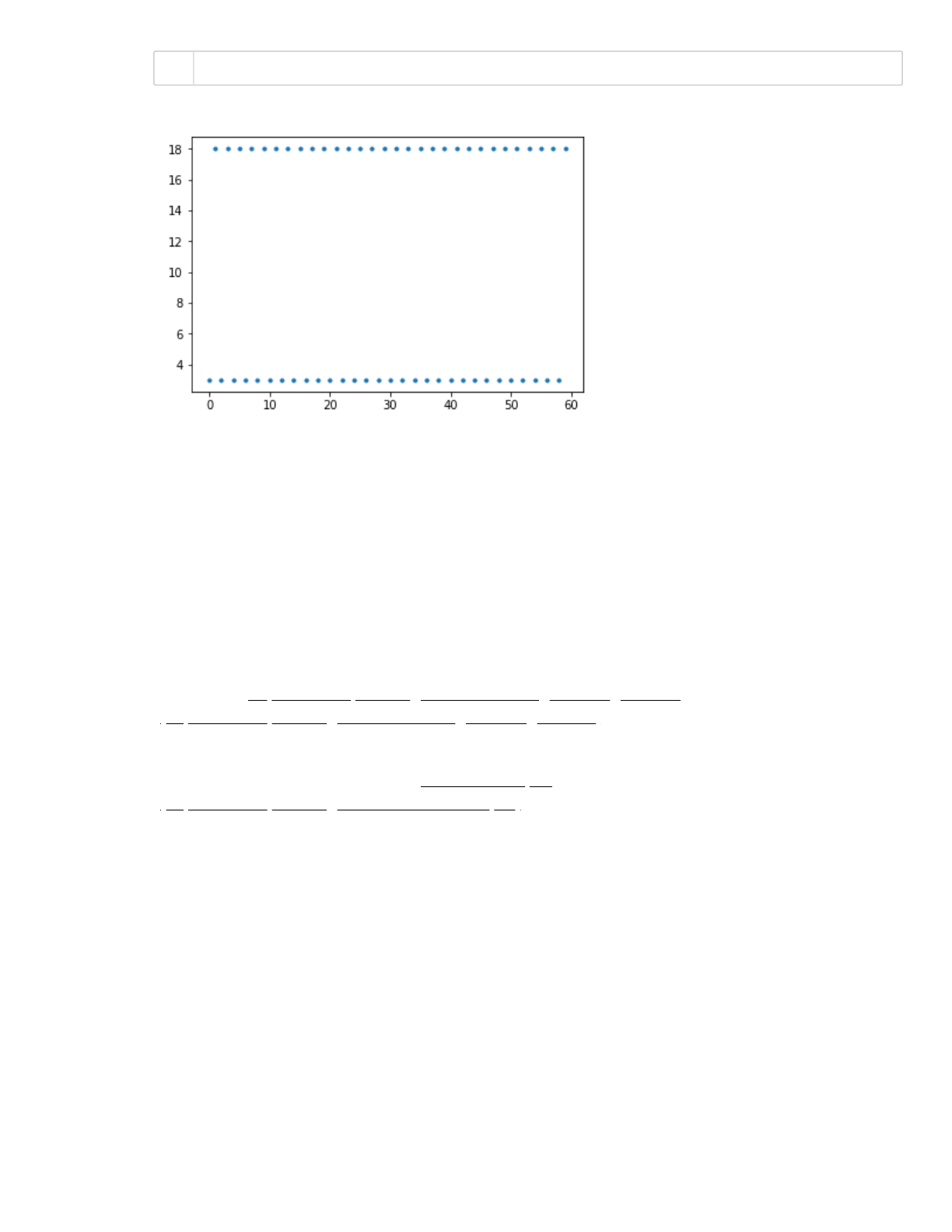
Notice there is a period, when numbers eventually start repeating. One of the advantages of the LCG
is that by using appropriate choice for the parameters, we can obtain known and long periods.
Check here https://en.wikipedia.org/wiki/Linear_congruential_generator
(https://en.wikipedia.org/wiki/Linear_congruential_generator) for a list of commonly used parameters
of LCGs.
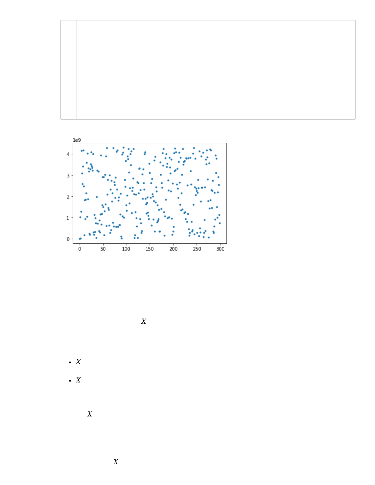
Let's try using the parameters from Numerical recipes
(https://en.wikipedia.org/wiki/Numerical_Recipes)
Out[9]:
[<matplotlib.lines.Line2D at 0x10e248eb8>]
plt.plot(x,'.')1
2/18/2020 MonteCarloMethods
localhost:8888/notebooks/GitCourseRepo/cs357-sp20/assets/demos/6-monte-carlo/MonteCarloMethods.ipynb#b)-Write-a-function-to-evaluate-the-probability-the-p
…
4/36
In[10]:
"Good" random number generators are efficient, have long peiods and are portable.
Random Variables
Think of a random variable as a function that maps the outcome of an unpredictable (random)
processses to numerical quantities.
For example:
= the face of a bread when it falls on the ground. The random value can abe the "buttered"
side or the "not buttered" side
= value that appears on top of dice after each roll
We don't have an exact number to represent these random processes, but we can get something
that represents the average case. To do that, we need to know the likelihood of each individual
value of .
Coin toss
Random variable : result of a coin toss
Out[10]:
[<matplotlib.lines.Line2D at 0x116a1ada0>]
s = 8
a = 1664525
c = 1013904223
m = 2**32
n = 300
x = np.zeros(n)
x[0] = s
for i in range(1,n):
x[i] = (a * x[i-1] + c) % m
plt.plot(x,'.')
1
2
3
4
5
6
7
8
9
10
11
12
2/18/2020 MonteCarloMethods
localhost:8888/notebooks/GitCourseRepo/cs357-sp20/assets/demos/6-monte-carlo/MonteCarloMethods.ipynb#b)-Write-a-function-to-evaluate-the-probability-the-p
…
5/36
In each toss, the random variable can take the values (tail) and (head), and each
has probability .
The expected value of a discrete random variable is defined as:
Hence for a coin toss we have:
Roll Dice
Random variable : value that appears on top of the dice after each roll
In each toss, the random variable can take the values and each has
probability .
The expected value of the discrete random variable is defined as:
In[11]:
Monte Carlo Methods
Monte Carlo methods are algorithms that rely on repeated random sampling to approximate a
desired quantity.
Example 1) Simulating a coin toss experiment
We want to find the probability of heads when tossing a coin. We know the expected value is 0.5.
Using Monte Carlo with N samples (here tosses), our estimate of the expected value is:
where if the toss gives head.
Let's toss a "fair" coin N times and record the results for each toss.
But first, how can we simulate one toss?
Out[11]:
3.5
E = 0
for i in range(6):
E += (i+1)*(1/6)
E
1
2
3
4
2/18/2020 MonteCarloMethods
localhost:8888/notebooks/GitCourseRepo/cs357-sp20/assets/demos/6-monte-carlo/MonteCarloMethods.ipynb#b)-Write-a-function-to-evaluate-the-probability-the-p
…
6/36
In[12]:
In[13]:
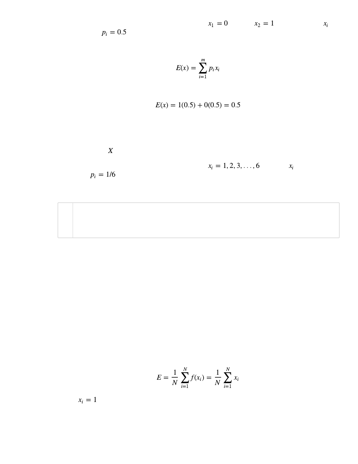
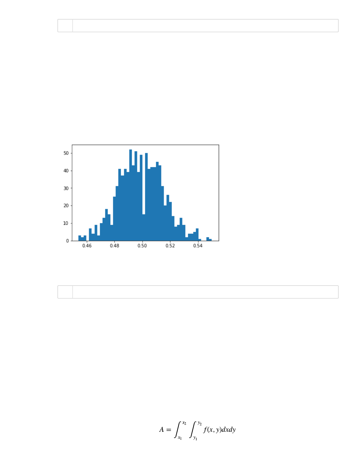
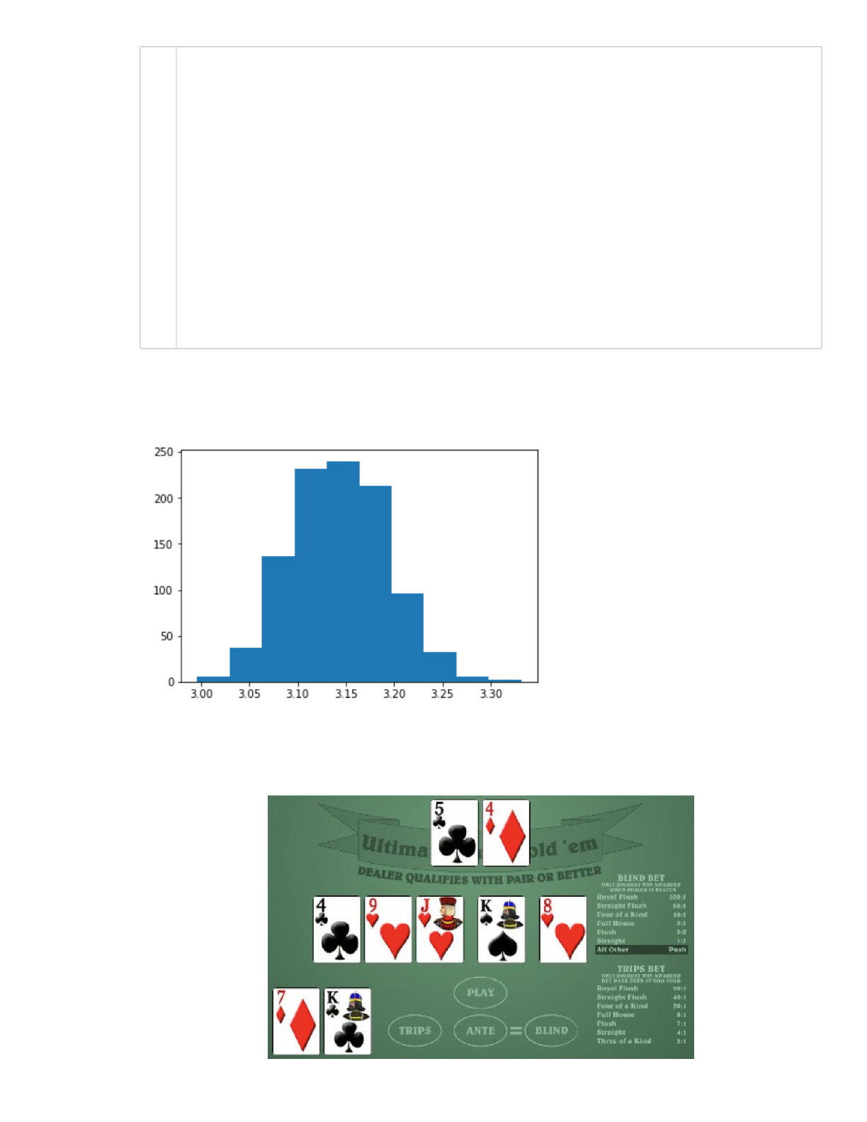
Note that if we run the code snippet above again, it is likely we will get a different result. What if we
run this many times?
In[14]:
0
Out[13]:
0.5
Out[14]:
(array([ 15., 39., 98., 210., 197., 220., 142., 53., 22., 4.]),
array([0.454 , 0.4636, 0.4732, 0.4828, 0.4924, 0.502 , 0.5116, 0.5212,
0.5308, 0.5404, 0.55 ]),
<a list of 10 Patch objects>)
toss = np.random.choice([0,1])
print(toss)
N = 30 # number of samples (tosses)
toss_list = []
for i in range(N):
toss = np.random.choice([0,1])
toss_list.append(toss)
np.array(toss_list).sum()/N
#clear
N = 1000 # number of tosses
M = 1000 # number of numerical experiments
nheads = []
for j in range(M):
toss_list = []
for i in range(N):
toss_list.append(np.random.choice([0,1]))
nheads.append( np.array(toss_list).sum()/N )
nheads = np.array(nheads)
plt.hist(nheads)
1
2
1
2
3
4
5
6
7
8
1
2
3
4
5
6
7
8
9
10
11
12
2/18/2020 MonteCarloMethods
localhost:8888/notebooks/GitCourseRepo/cs357-sp20/assets/demos/6-monte-carlo/MonteCarloMethods.ipynb#b)-Write-a-function-to-evaluate-the-probability-the-p
…
7/36
In[15]:
In[16]:
What happens when we increase the number of numerical experiments?
Monte Carlo to approximate integrals
One of the most important applications of Monte Carlo methods is in estimating volumes and areas
that are difficult to compute analytically. Without loss of generality we will first present Monte Carlo
to approximate two-dimensional integrals. Nonetheless, Monte Carlo is a great method to solve
high-dimensional problems.
To approximate an integration
Out[15]:
(array([ 3., 2., 3., 0., 7., 4., 9., 3., 10., 13., 18., 15., 9.,
25., 31., 41., 37., 41., 39., 52., 43., 51., 39., 49., 15., 50.,
41., 42., 42., 45., 43., 31., 20., 26., 22., 14., 8., 9., 13.,
9., 2., 4., 4., 5., 7., 1., 0., 0., 2., 1.]),
array([0.454 , 0.45592, 0.45784, 0.45976, 0.46168, 0.4636 , 0.46552,
0.46744, 0.46936, 0.47128, 0.4732 , 0.47512, 0.47704, 0.47896,
0.48088, 0.4828 , 0.48472, 0.48664, 0.48856, 0.49048, 0.4924 ,
0.49432, 0.49624, 0.49816, 0.50008, 0.502 , 0.50392, 0.50584,
0.50776, 0.50968, 0.5116 , 0.51352, 0.51544, 0.51736, 0.51928,
0.5212 , 0.52312, 0.52504, 0.52696, 0.52888, 0.5308 , 0.53272,
0.53464, 0.53656, 0.53848, 0.5404 , 0.54232, 0.54424, 0.54616,
0.54808, 0.55 ]),
<a list of 50 Patch objects>)
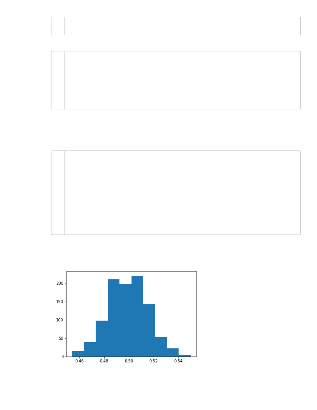
0.498925 0.016231062041653355
plt.hist(nheads, bins=50)
print(nheads.mean(),nheads.std())
1
1
2/18/2020 MonteCarloMethods
localhost:8888/notebooks/GitCourseRepo/cs357-sp20/assets/demos/6-monte-carlo/MonteCarloMethods.ipynb#b)-Write-a-function-to-evaluate-the-probability-the-p
…
8/36
we sample points uniformily inside a domain , i.e. we let be a uniformily
distributed random variable on .
Using Monte Carlo with N sample points, our estimate for the expected value (that a sample point is
inside the circle) is:
which gives the approximate for the integral:
Law of large numbers:
as , the sample average converges the the expected value and hence
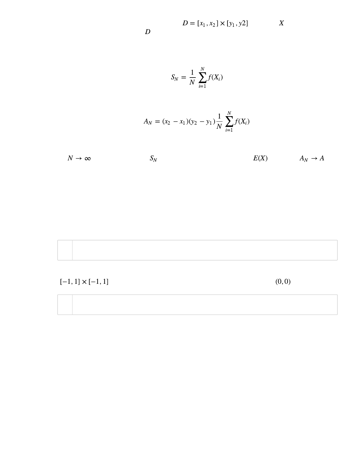
Example 2) Approximate the area of a circle
We will use Monte Carlo Method to approximate the area of a circle of radius R = 1.
Let's start with a uniform distribution on the unit square [0,1]×[0,1] . Create a 2D array samples of
shape (2, N):
In[17]:
Scale the sample points "samples", so that we have a uniform distribution inside a square
. Calculate the distance from each sample point to the origin
In[18]:
N = 10**2
samples = np.random.rand(2, N)
xy = samples * 2 - 1.0 # scale sample points
r = np.sqrt(xy[0, :]**2 + xy[1, :]**2) # calculate radius
1
2
1
2

2/18/2020 MonteCarloMethods
localhost:8888/notebooks/GitCourseRepo/cs357-sp20/assets/demos/6-monte-carlo/MonteCarloMethods.ipynb#b)-Write-a-function-to-evaluate-the-probability-the-p
…
9/36
In[19]:
We then count how many of these points are inside the circle centered at the origin.
In[20]:
And the approximated value for the area is:
In[21]:
We can assign different colors to the points inside the circle and plot (just for vizualization purposes).
69
Out[21]:
2.76
plt.plot(xy[0,:], xy[1,:], 'k.')
plt.axis('equal')
plt.xlabel('x')
plt.ylabel('y');
incircle = (r <= 1)
count_incircle = incircle.sum()
print(count_incircle)
A_approx = (2*2) * (count_incircle)/N
A_approx
1
2
3
4
1
2
3
1
2
2/18/2020 MonteCarloMethods
localhost:8888/notebooks/GitCourseRepo/cs357-sp20/assets/demos/6-monte-carlo/MonteCarloMethods.ipynb#b)-Write-a-function-to-evaluate-the-probability-the-
…
10/36
In[22]:
Combine all the relevant code above, so we can easily run this numerical experiment for different
sample size N.
In[23]:
Perform the same above, but now store the approximated area for different N, and plot:
In[24]:
The approximated area is:
3.28
plt.plot(xy[0,np.where(incircle)[0]], xy[1,np.where(incircle)[0]], 'b.')
plt.plot(xy[0,np.where(incircle==False)[0]], xy[1,np.where(incircle==Fal
plt.axis('equal')
plt.xlabel('x')
plt.ylabel('y');
#clear
N = 10**2
samples = np.random.rand(2, N)
xy = samples * 2 - 1.0 # scale sample points
r = np.sqrt(xy[0, :]**2 + xy[1, :]**2) # calculate radius
incircle = (r <= 1)
count_incircle = incircle.sum()
A_approx = (2*2) * (count_incircle)/N
print(A_approx)
#clear
N = 10**6
samples = np.random.rand(2, N)
xy = samples * 2 - 1.0 # scale sample points
r = np.sqrt(xy[0, :]**2 + xy[1, :]**2) # calculate radius
incircle = (r <= 1)
N_samples = np.arange(1,N+1)
A_approx = 4 * incircle.cumsum() / N_samples
1
2
3
4
5
1
2
3
4
5
6
7
8
9
1
2
3
4
5
6
7
8
2/18/2020 MonteCarloMethods
localhost:8888/notebooks/GitCourseRepo/cs357-sp20/assets/demos/6-monte-carlo/MonteCarloMethods.ipynb#b)-Write-a-function-to-evaluate-the-probability-the-
…
11/36
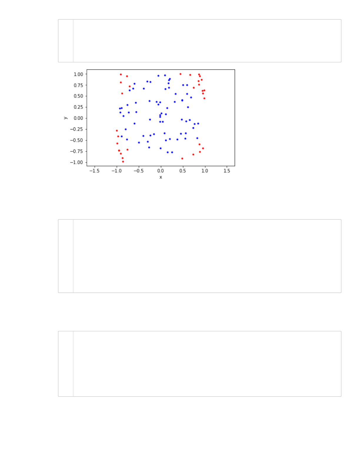
In[25]:
In[26]:
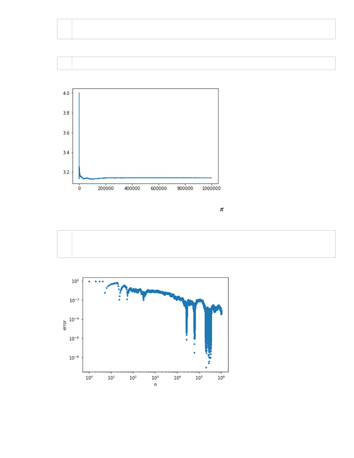
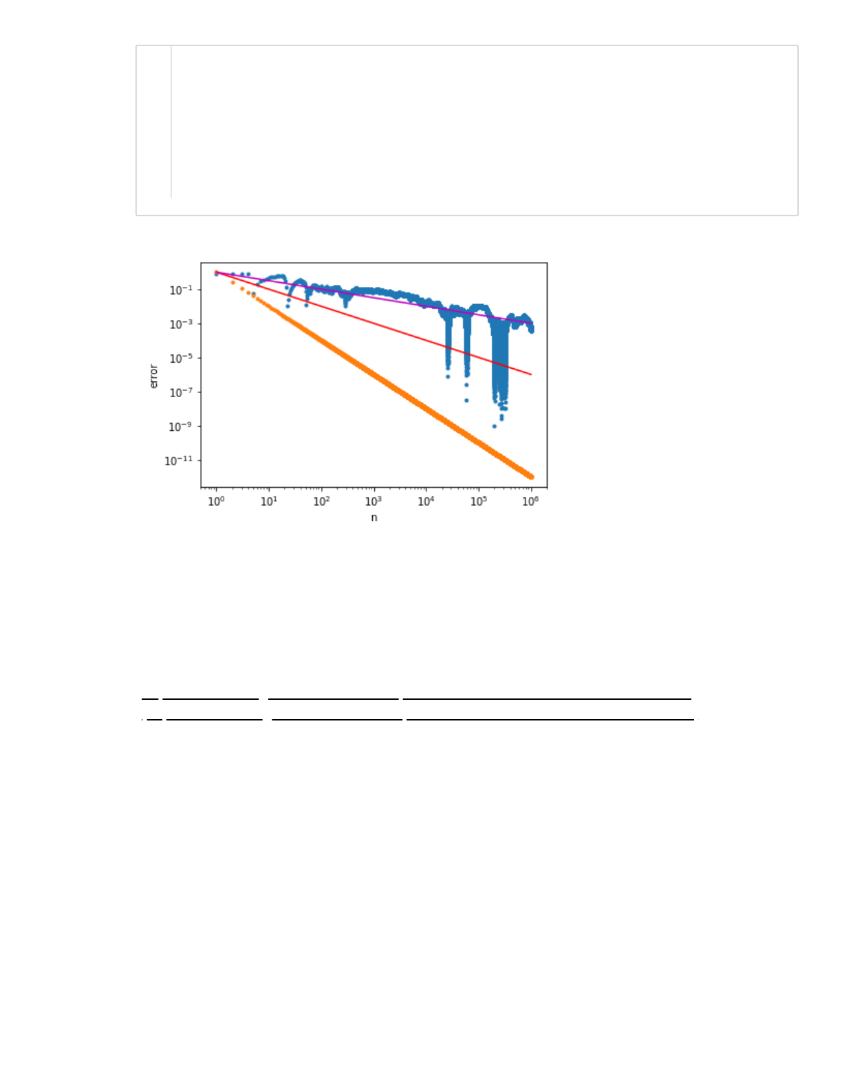
Which as expected gives an approximation for the number , since the circle has radius 1. Let's plot
the error of our approximation:
In[27]:
Out[25]:
3.142012
Out[26]:
[<matplotlib.lines.Line2D at 0x116e0b390>]
Out[27]:
Text(0, 0.5, 'error')
#clear
A_approx[-1]
plt.plot(A_approx)
plt.loglog(N_samples, np.abs(A_approx - np.pi), '.')
plt.xlabel('n')
plt.ylabel('error')
1
2
1
1
2
3
2/18/2020 MonteCarloMethods
localhost:8888/notebooks/GitCourseRepo/cs357-sp20/assets/demos/6-monte-carlo/MonteCarloMethods.ipynb#b)-Write-a-function-to-evaluate-the-probability-the-
…
12/36
In[28]:
More for errors of Monte Carlo methods here:
https://courses.engr.illinois.edu/cs357/sp2020/references/ref-4-random-monte-carlo/
(https://courses.engr.illinois.edu/cs357/sp2020/references/ref-4-random-monte-carlo/)
Out[28]:
[<matplotlib.lines.Line2D at 0x1213412b0>]
plt.loglog(N_samples, np.abs(A_approx - np.pi), '.')
plt.xlabel('n')
plt.ylabel('error')
plt.loglog(N_samples, 1/N_samples**2, '.')
plt.loglog(N_samples, 1/N_samples, 'r')
plt.loglog(N_samples, 1/np.sqrt(N_samples), 'm')
1
2
3
4
5
6
7
8
2/18/2020 MonteCarloMethods
localhost:8888/notebooks/GitCourseRepo/cs357-sp20/assets/demos/6-monte-carlo/MonteCarloMethods.ipynb#b)-Write-a-function-to-evaluate-the-probability-the-
…
13/36
In[29]:
Example 3) Approximating probabilities of a Poker game
Out[29]:
(array([ 6., 37., 136., 232., 240., 213., 96., 32., 6., 2.]),
array([2.996 , 3.0296, 3.0632, 3.0968, 3.1304, 3.164 , 3.1976, 3.2312,
3.2648, 3.2984, 3.332 ]),
<a list of 10 Patch objects>)
N = 10**3
M = 1000
A_list = []
for i in range(M):
samples = np.random.rand(2, N)
xy = samples * 2 - 1.0 # scale sample points
r = np.sqrt(xy[0, :]**2 + xy[1, :]**2) # calculate radius
incircle = (r <= 1)
count_incircle = incircle.sum()
A_list.append( (2*2) * (count_incircle)/N )
A_array = np.array(A_list)
plt.hist(A_list)
1
2
3
4
5
6
7
8
9
10
11
12
13
14
15
16

2/18/2020 MonteCarloMethods
localhost:8888/notebooks/GitCourseRepo/cs357-sp20/assets/demos/6-monte-carlo/MonteCarloMethods.ipynb#b)-Write-a-function-to-evaluate-the-probability-the-
…
14/36
What is the probability of winning a hand of Texas Holdem for a given starting hand? This is a non-
trivial problem to solve analytically, specially if you include many players and the chances that a
player will fold (give-up) before the end of a round of cards. Let's use Monte Carlo Methods to
approximate these probabilities!
Assumptions:
You are playing against only one player (the opponent)
Both players stay until the end of a game (all 5 dealer cards), so players do not fold.
Monte Carlo simulation: for a given "starting hand" that we wish to obtain the winning probability,
generate a set of N games and use the Texas Holdem rules to decide who wins (starting hand,
opponent or there is a tie).
A game is a set of 7 random cards: 2 cards for opponent + 5 cards for the dealer.
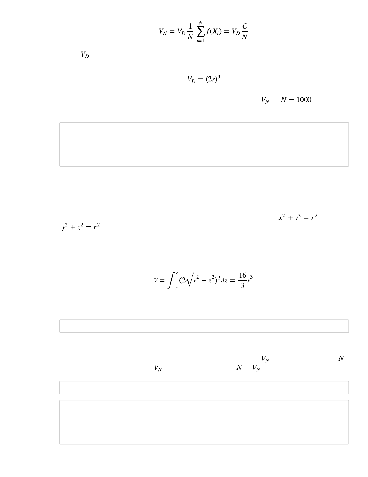
For example, suppose the starting hand is 5 of clubs and 4 of diamonds. You perform N=1000
games, and counts 350 wins, 590 losses and 60 ties. Your numerical experiment estimated a
probability of winning of 35%.
This is your first MP!
Example 4) Calculating a Volume of Intersection
In this exercise, we will use Monte Carlo integration to compute a volume of intersection between
two cylinders. This integral is possible to compute analytically, so we can compare our answer to the
true result and see how accurate it is.
The solid common to two right circular cylinders of equal radii intersecting at right angles is called
the Steinmetz solid.
Two cylinders intersecting at right angles are called a bicylinder or mouhefanggai (Chinese for "two
square umbrellas").
http://mathworld.wolfram.com/SteinmetzSolid.html
(http://mathworld.wolfram.com/SteinmetzSolid.html)
To help you check if you are going in the right direction, you can copy the functions you define here
inside PrairieLearn.
https://prairielearn.engr.illinois.edu/pl/course_instance/52088/assessments
(https://prairielearn.engr.illinois.edu/pl/course_instance/52088/assessments)

2/18/2020 MonteCarloMethods
localhost:8888/notebooks/GitCourseRepo/cs357-sp20/assets/demos/6-monte-carlo/MonteCarloMethods.ipynb#b)-Write-a-function-to-evaluate-the-probability-the-
…
15/36
a) Write a function that will determine if a given point is inside both cylinders
Write the function insideCylinders that given a NumPy array representing some arbitrary point in
a 3-dimensional space returns true if the point is inside both cylinders. Assume the solid is
centered at the origin and that both cylinders have radius .
def insideCylinders(pos,r):
# pos = np.array([x,y,z])
# r = radius of the cylinders
return bool
In[30]:
b) Write a function to evaluate the probability the point is inside the given volume
The function prob_inside_volume should take as argument the number of random points N.
The function generate N random points inside a box around the intersection of the cylinders, and
uses the function insideCylinders to determine if the point is inside the cylinders or not. Recall
that these random points should be generated in a form of a NumPy array.
Track the number of points that fall inside both cylinders. Return the ratio as a floating point
number.
def prob_inside_volume(N,r):
# N = number of sample points
# r = radius of the cylinders
return float
In[31]:
c) Use the ratio to estimate the volume of intersection
To approximate the volume of the intersection, we use:
#clear
def insideCylinders(pos, r):
return ((pos[0]** 2 + pos[1]** 2) <= r) and ((pos[1]** 2 + pos[2]**
#clear
def prob_inside_volume(N,r):
C = 0.0
for i in range(N):
x = random.uniform(-r, r)
y = random.uniform(-r, r)
z = random.uniform(-r, r)
pos = np.array([x,y,z])
if (insideCylinders(pos,r)):
C += 1
return C / N
1
2
3
1
2
3
4
5
6
7
8
9
10
11
2/18/2020 MonteCarloMethods
localhost:8888/notebooks/GitCourseRepo/cs357-sp20/assets/demos/6-monte-carlo/MonteCarloMethods.ipynb#b)-Write-a-function-to-evaluate-the-probability-the-
…
16/36
where is the volume of the domain used to generate the sample points. In this example, we
considered the domain as the box around the intersection of the cylinders, hence
Use your function prob_inside_volume to approximate the volume for for
cylinders of radius 1.
In[32]:
d) Comparing with the exact solution
Two cylinders of radius r oriented long the z- and x-axes gives the equations and
The volume common to two cylinders was known to Archimedes and the Chinese mathematician
Tsu Ch'ung-Chih, and does not require calculus to derive. Using calculus provides a simple
derivation, however. The volume is given by
Compare your approximated result above with the exact volume.
In[33]:
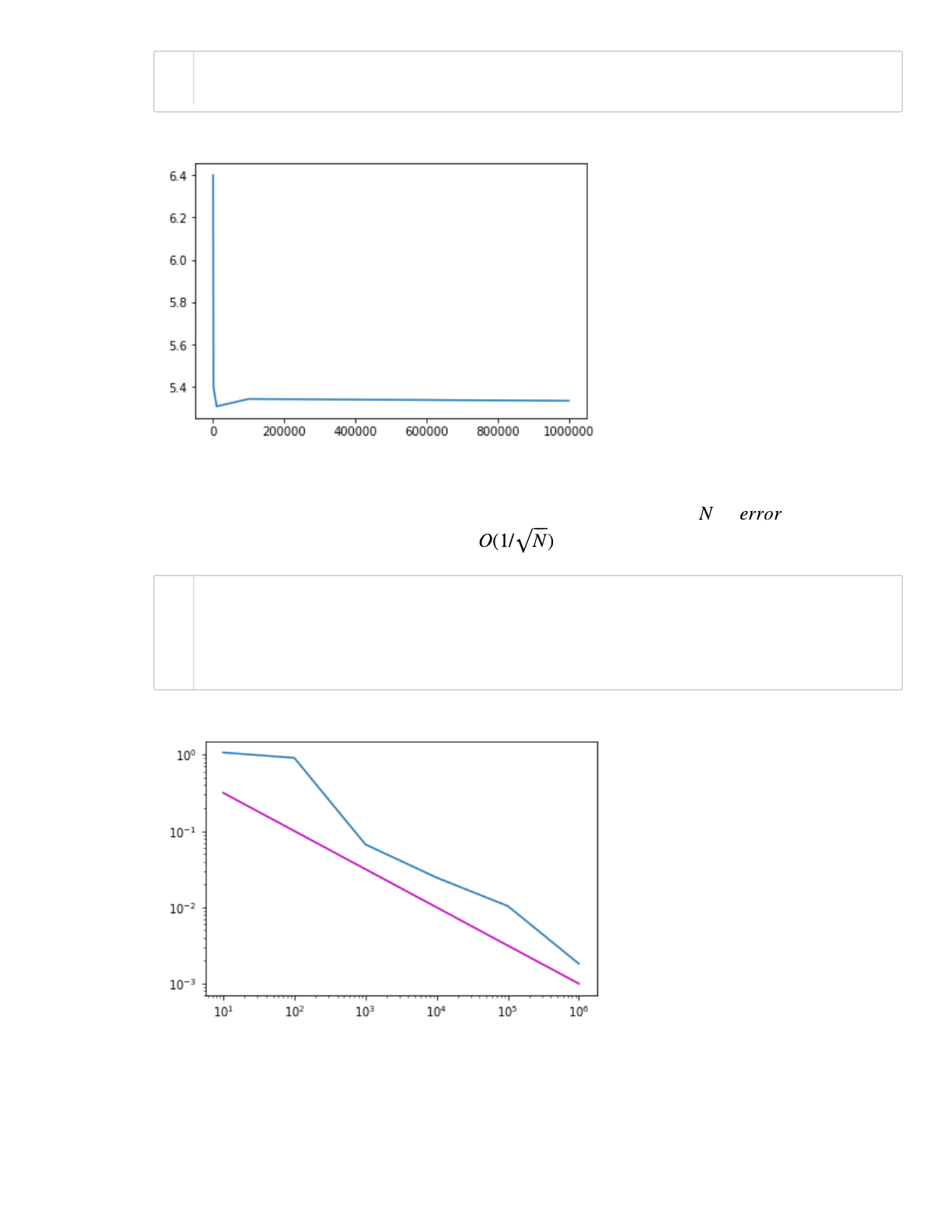
Use your function prob_inside_volume to approximate the volume for increasing values of
defined in Nvalues. Store each in a list approxVol. Plot vs .
In[34]:
In[35]:
5.256
Out[33]:
5.333333333333333
#clear
N = 1000
r = 1
Vn = prob_inside_volume(N,r)*(2*r)**3
print(Vn)
16/3
Nvalues = [(10**N) for N in range(1,7)]
#clear
approxVol = []
for N in Nvalues:
approxVol.append( prob_inside_volume(N,r) * (2*r)**3 )
1
2
3
4
5
1
1
1
2
3
4
5
2/18/2020 MonteCarloMethods
localhost:8888/notebooks/GitCourseRepo/cs357-sp20/assets/demos/6-monte-carlo/MonteCarloMethods.ipynb#b)-Write-a-function-to-evaluate-the-probability-the-
…
17/36
In[36]:
Compute the absolute error, using the exact expression given above. Plot vs . Compare with
the known asymptotic behavior of the error
In[37]:
Random Walk
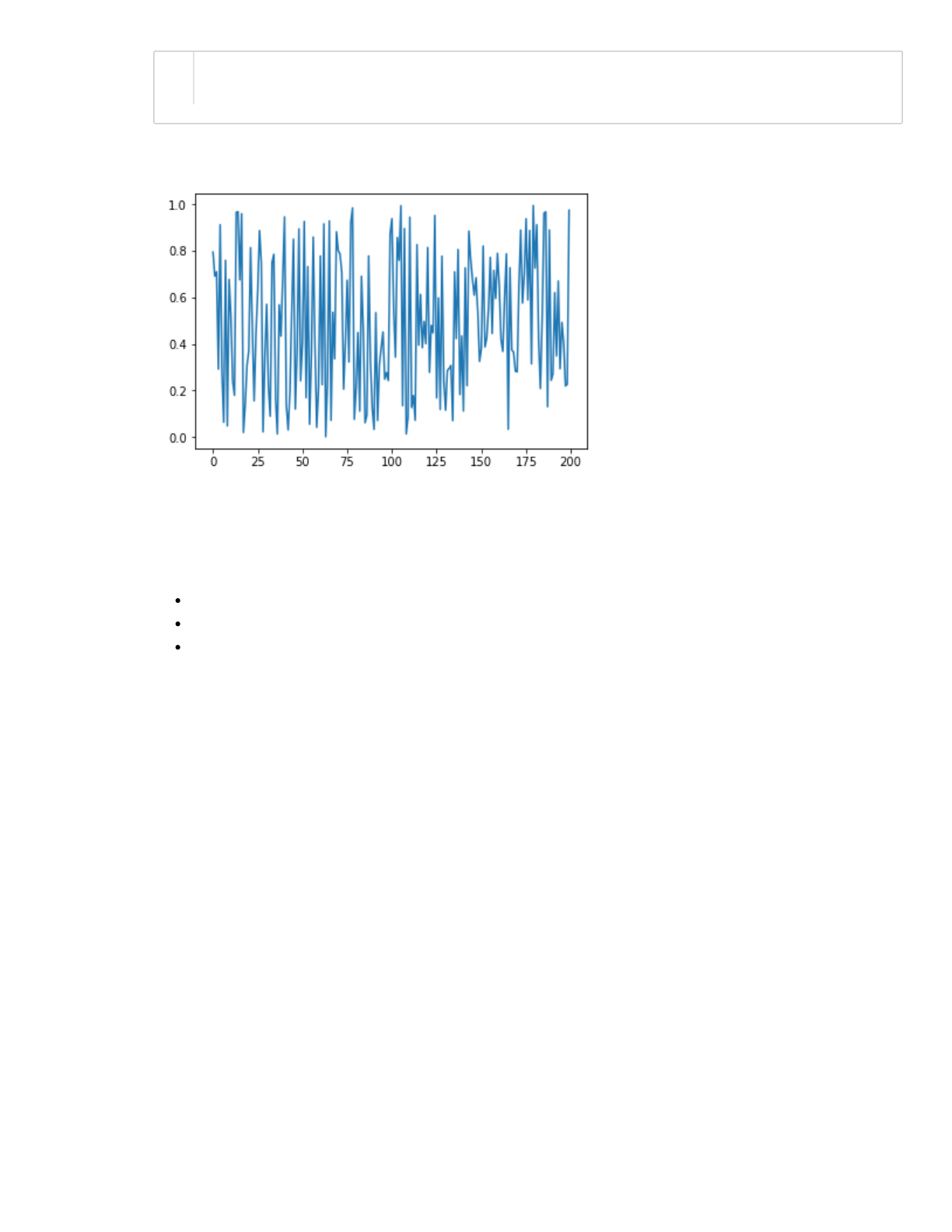
First we will generate a list of random numbers and plot:
Out[36]:
[<matplotlib.lines.Line2D at 0x116e47cf8>]
Out[37]:
[<matplotlib.lines.Line2D at 0x137263828>]
#clear
plt.plot(Nvalues,approxVol)
#clear
r = 1
trueVol = (16.0/3.0)*r**3
plt.loglog(Nvalues,np.abs(np.array(approxVol)-trueVol))
plt.loglog(Nvalues, 1/np.sqrt(Nvalues), 'm')
1
2
1
2
3
4
5
2/18/2020 MonteCarloMethods
localhost:8888/notebooks/GitCourseRepo/cs357-sp20/assets/demos/6-monte-carlo/MonteCarloMethods.ipynb#b)-Write-a-function-to-evaluate-the-probability-the-
…
18/36
In[38]:
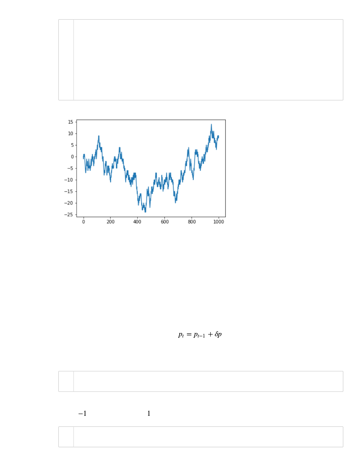
A random walk is different from a list of random numbers because the next value in the sequence is
a modification of the previous value in the sequence. Here is simple model of a random walk:
Start with a random number of either -1 or 1.
Randomly select a -1 or 1 and add it to the observation from the previous time step.
Repeat step 2 for as long as you like.
Create the array rand_walk with N = 1000 points using the algorithm above. Plot the array.
Out[38]:
[<matplotlib.lines.Line2D at 0x1213415f8>]
series = np.random.rand(200)
plt.plot(series)
1
2
2/18/2020 MonteCarloMethods
localhost:8888/notebooks/GitCourseRepo/cs357-sp20/assets/demos/6-monte-carlo/MonteCarloMethods.ipynb#b)-Write-a-function-to-evaluate-the-probability-the-
…
19/36
In[39]:
Example 5) Modeling stock prices (simple model)
Suppose that we are interested in investing in a specific stock. We may want to try and predict what
the future price might be with some probability in order for us to determine whether or not we should
invest.
The simplest way to model the movement of the price of an asset in a market with no moving forces
is to assume that the price changes with some random magnitude and direction, following a random
walk model.
We model the magnitude of the price change with the roll of a die. The function dice "rolls" an
integer number from 1 to 6.
In[40]:
To model prices increasing or decreasing, we will use the "flip" of a coin. The function flip returns
either (decreasing price) or (increasing price).
In[41]:
Out[39]:
[<matplotlib.lines.Line2D at 0x137428588>]
#clear
N = 1000
rand_walk = [0]
for i in range(N-1):
step = np.random.choice([-1,1])
rand_walk.append( rand_walk[-1]+step)
rand_walk = np.array(rand_walk)
plt.plot(rand_walk)
def dice():
return np.random.randint(1,7)
def flip():
return np.random.choice([1, -1])
1
2
3
4
5
6
7
8
9
10
1
2
1
2
2/18/2020 MonteCarloMethods
localhost:8888/notebooks/GitCourseRepo/cs357-sp20/assets/demos/6-monte-carlo/MonteCarloMethods.ipynb#b)-Write-a-function-to-evaluate-the-probability-the-
…
20/36
By combining these two functions, we are able to obtain the price change at a given time. Here we
will assume that a coin flip combined with a dice roll gives the price change for a given day.
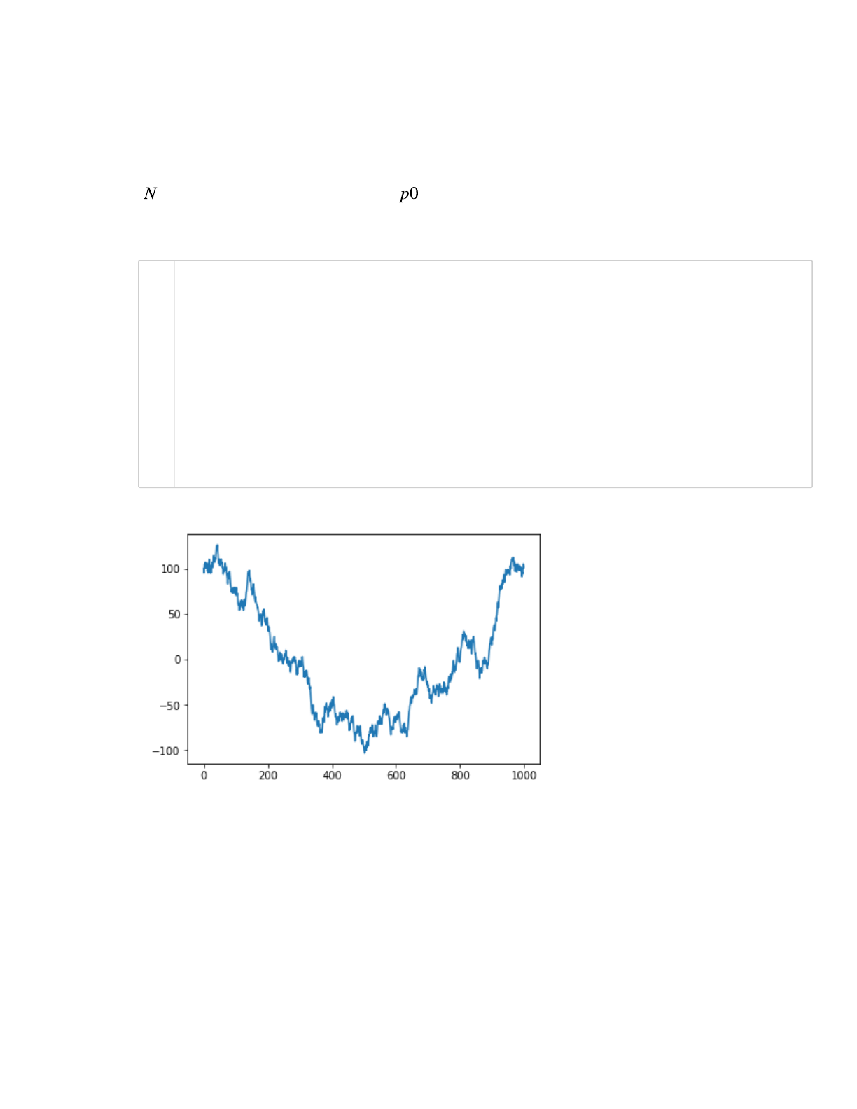
a) Performing one numerical experiment:
Use the random walk model described above to predict the asset price for each day over a period of
days. The initial price of the stock is . Store the price per day in the numpy array price.
For now, use N = 1000 and p0 = 100.
In[42]:
Does this plot resemble the short-term movement of the stock market?
Observations:
Performing one time step per day may not be enough to fully capture the randomness of the motion
of the market. In practice, these N steps would really represent what the price might be in some
shorter period of time (much less than a whole day).
Furthermore, performing a single numerical experiment will not give us a realistic expectation of
what the price of the stock might be after a certain amount of time since the stock market with no
moving forces consists of random movements.
Out[42]:
[<matplotlib.lines.Line2D at 0x137548278>]
#clear
N = 1000
p0 = 100
price = [p0]
for i in range(N-1):
step = flip()*dice()
price.append( price[-1]+step)
price = np.array(price)
plt.plot(price)
1
2
3
4
5
6
7
8
9
10
11
12

2/18/2020 MonteCarloMethods
localhost:8888/notebooks/GitCourseRepo/cs357-sp20/assets/demos/6-monte-carlo/MonteCarloMethods.ipynb#b)-Write-a-function-to-evaluate-the-probability-the-
…
21/36
Run the code snippet above several times (just do shift-enter again and again). What happens to the
asset price after N days?
We will be running several numerical experiments that simulates the price variation over N days.
Wrap the code snippet above in the function simulate_asset_price that takes N and p0 as
argument and returns the array price.
In[43]:
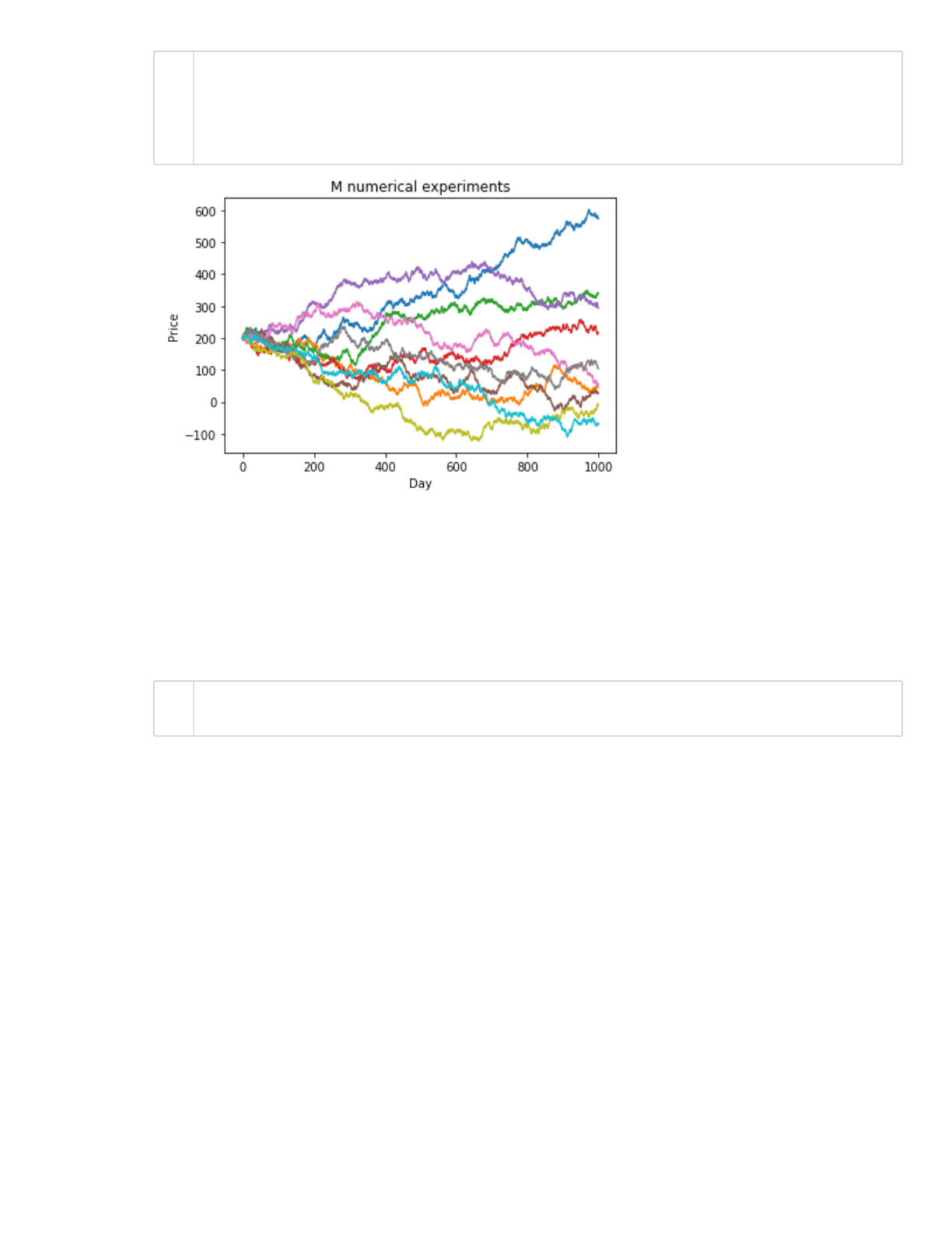
b) Performing M=10 different numerical experiments, each one with N = 1000 days
For each numerical experiment, use the function simulate_asset_price with N = 1000 and p0
= 200.
Store all the M=10 arrays price in the 2d array prices_M with shape (N,M)
In[44]:
In[45]:
Then you can plot your results using:
#clear
def simulate_asset_price(N,p0):
price = [p0]
for i in range(N-1):
step = flip()*dice()
price.append( price[-1]+step)
return np.array(price)
N = 1000 # days
M = 10 # number of numerical experiments
p0 = 200 # initial asset price
#clear
price_M = []
for i in range(M):
price = simulate_asset_price(N,p0)
price_M.append(price)
price_M = np.array(price_M).T
1
2
3
4
5
6
7
1
2
3
1
2
3
4
5
6
2/18/2020 MonteCarloMethods
localhost:8888/notebooks/GitCourseRepo/cs357-sp20/assets/demos/6-monte-carlo/MonteCarloMethods.ipynb#b)-Write-a-function-to-evaluate-the-probability-the-
…
22/36
In[46]:
We now have a more insightful prediction as to what the price of a given stock might be in the
future. Suppose we want to predict the asset price at day 1000. We can just take the last element of
the numpy array price!
Create the variable predicted_prices to store the predicted asset prices for day 1000 for all the
M=10 numerical experiments.
In[47]:
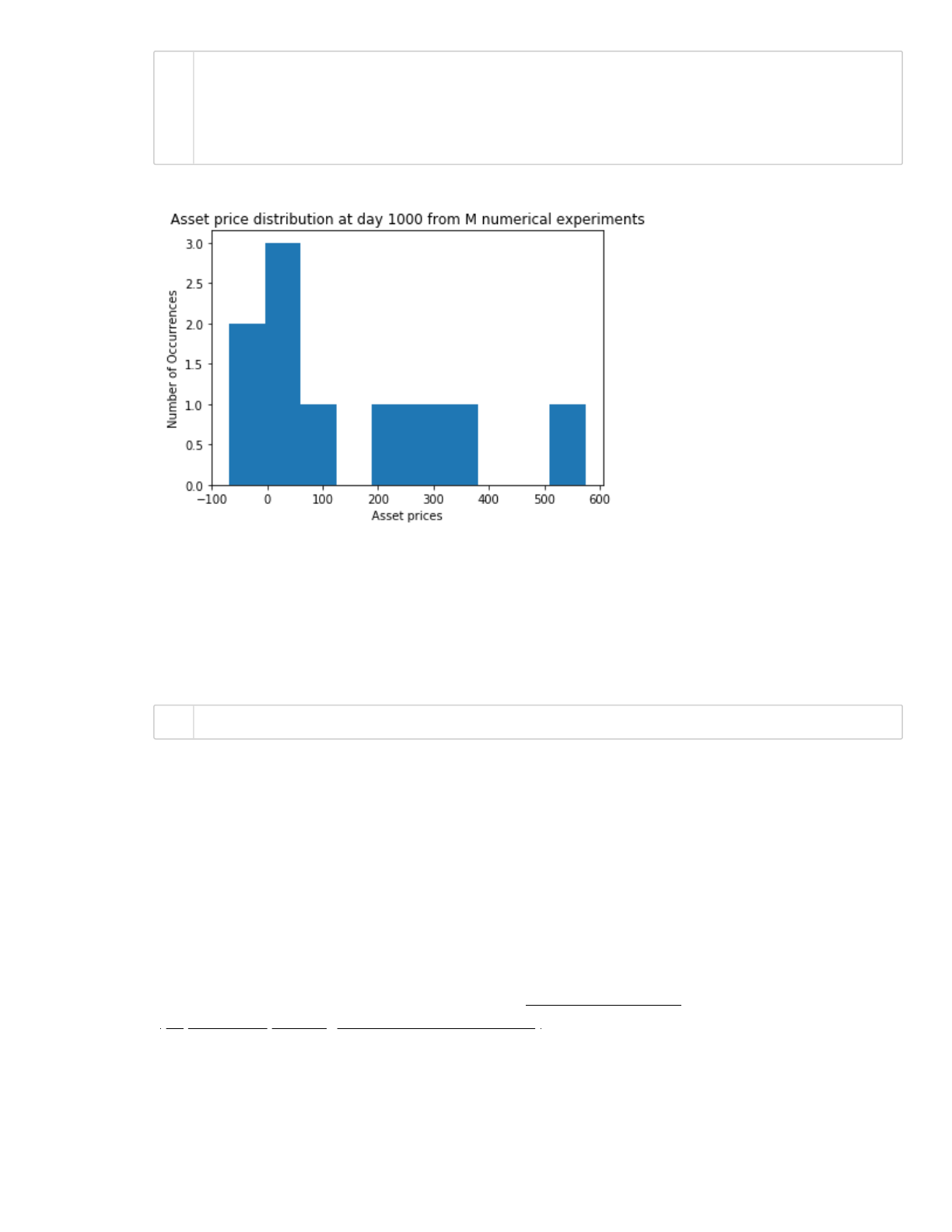
Plot the histogram of the predicted price:
plt.figure()
plt.plot(price_M);
plt.title ('M numerical experiments');
plt.xlabel('Day');
plt.ylabel('Price');
#clear
predicted_prices = price_M[-1,:]
1
2
3
4
5
1
2
2/18/2020 MonteCarloMethods
localhost:8888/notebooks/GitCourseRepo/cs357-sp20/assets/demos/6-monte-carlo/MonteCarloMethods.ipynb#b)-Write-a-function-to-evaluate-the-probability-the-
…
23/36
In[48]:
Go back and change the number of numerical experiments. Set M = 1000 and run again. Better
right?
You can calculate the mean of the distribution to get the “expected value” for the stock on day 1000.
What do you get?
In[49]:
There is one problem with our simple model. Our model does not incorporate any information about
our specific stock other than the starting price. In order for us to get a more accurate model, we
need to find a way incorporate the previous price of the stock. In the next example, we explore
another model for stock price behavior.
Example 6) Modeling stock prices (Black-Scholes Model)
We will now model stock price behavior using the Black-Scholes model
(https://en.wikipedia.org/wiki/Black_Scholes_model), which employs a type of log-normal
distribution to represent the growth of the stock price. Conceptually, this representation consists of
two pieces:
a) Growth based on interest rate only
b) Volatility of the market
Out[48]:
Text(0, 0.5, 'Number of Occurrences')
Out[49]:
158.0
plt.figure()
plt.hist(predicted_prices);
plt.title('Asset price distribution at day 1000 from M numerical experim
plt.xlabel('Asset prices')
plt.ylabel('Number of Occurrences')
predicted_prices.mean()
1
2
3
4
5
1
2/18/2020 MonteCarloMethods
localhost:8888/notebooks/GitCourseRepo/cs357-sp20/assets/demos/6-monte-carlo/MonteCarloMethods.ipynb#b)-Write-a-function-to-evaluate-the-probability-the-
…
24/36
Stock prices evolve over time, with a magnitude dependent on their volatility. The Black Scholes
model treats this evolution in terms of a random walk. To use the Black-Scholes model we assume:
some volatility of stock price. Call this
a (risk-free) interest rate called ; and
the price of the asset is geometric Brownian motion
(https://en.wikipedia.org/wiki/Geometric_Brownian_motion), or in other words the log of the
random process is a normal distribution.
which leads to the following expression for the predicted asset price:
meaning are normally distributed with mean and variance , where
is the volatility, or standard deviation on returns.
is a random value sampled from the normal distribution
price of the asset at time
initial price of the asset
is the interest rate
To predict the asset price at time , we will discretize the total time to maturity in small steps . For
each increment, we will use:
For example, if we want to obtain the asset price after 30 days, and we use the assumption that
prices change with the increment of one day, then our total number of price estimates is ,
and .
Write the function St_GBM that will compute the price of an asset at time given the
parameters ( )
def St_GBM(St, r, sigma, deltat):
St_next = ... # Calculate this
return St_next
In[50]:
This model now gives us a more accurate way to predict the future price.
Assume that at the initial time the asset price is , the interest rate is and
volatity is .
#clear
def St_GBM(St, r, sigma,deltat):
epsilon = deltat**0.5*sigma*np.random.normal()
S = St * np.exp( (r-sigma**2/2)*deltat + epsilon)
return S
1
2
3
4
5
2/18/2020 MonteCarloMethods
localhost:8888/notebooks/GitCourseRepo/cs357-sp20/assets/demos/6-monte-carlo/MonteCarloMethods.ipynb#b)-Write-a-function-to-evaluate-the-probability-the-
…
25/36
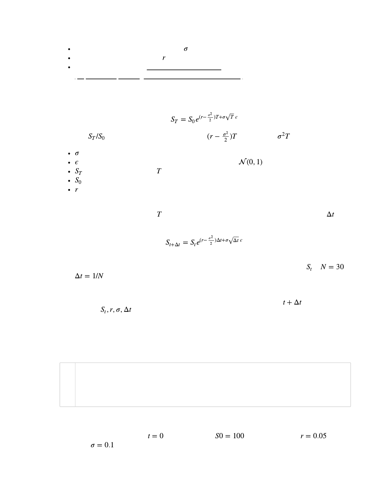
Calculate the daily price movements using St_GBM for a period of 252 days (typical number of
trading days in a year). Store your results in the array price. Then plot your results using
plt.plot(price)
In[51]:
Unfortunately volatility is usually not this small.... Run the code snippet above to predict the
price movement for a volatity
We have managed to successfully simulate a year’s worth of future daily price data. Unfortunately
this does not provide insight into risk and return characteristics of the stock as we only have one
randomly generated path. The likelyhood of the actual price evolving exactly as described in the
above charts is pretty much zero. We should modify the above code to run multiple numerical
experiments (or simulations).
Perform M=10 different numerical experiments, each one with N = 252 days
For each numerical experiment, determine the array price using N = 252 days. Make sure to store
Out[51]:
Text(0, 0.5, 'Price')
#clear
N = 252 # number of days
S0 = 100
r = 0.05
sigma = 0.1
deltaT = 1/N
price = np.array([S0])
for i in range(N):
st = price[-1]
price = np.append(price, St_GBM(price[-1],r,sigma,deltaT) )
plt.plot(price)
plt.title('Simulation of Price using Black-Scholes Model')
plt.xlabel('Time')
plt.ylabel('Price')
1
2
3
4
5
6
7
8
9
10
11
12
13
14
15
16
2/18/2020 MonteCarloMethods
localhost:8888/notebooks/GitCourseRepo/cs357-sp20/assets/demos/6-monte-carlo/MonteCarloMethods.ipynb#b)-Write-a-function-to-evaluate-the-probability-the-
…
26/36
all the M=10 arrays price in the 2d array prices_M.
For this sequence of numerical experiments, assume that the initial asset price is S0 = 100.
In[52]:
In[53]:
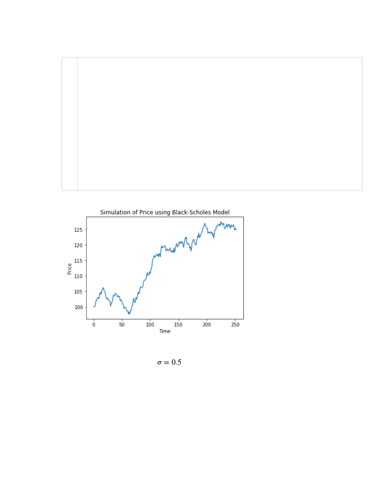
Then plot the result using:
In[54]:
The spread of final prices is quite large! Let's take a further look at this spread. Create the variable
predicted_prices to store the predicted asset prices for day 252 (last day) for all the M=10
numerical experiments.
In[55]:
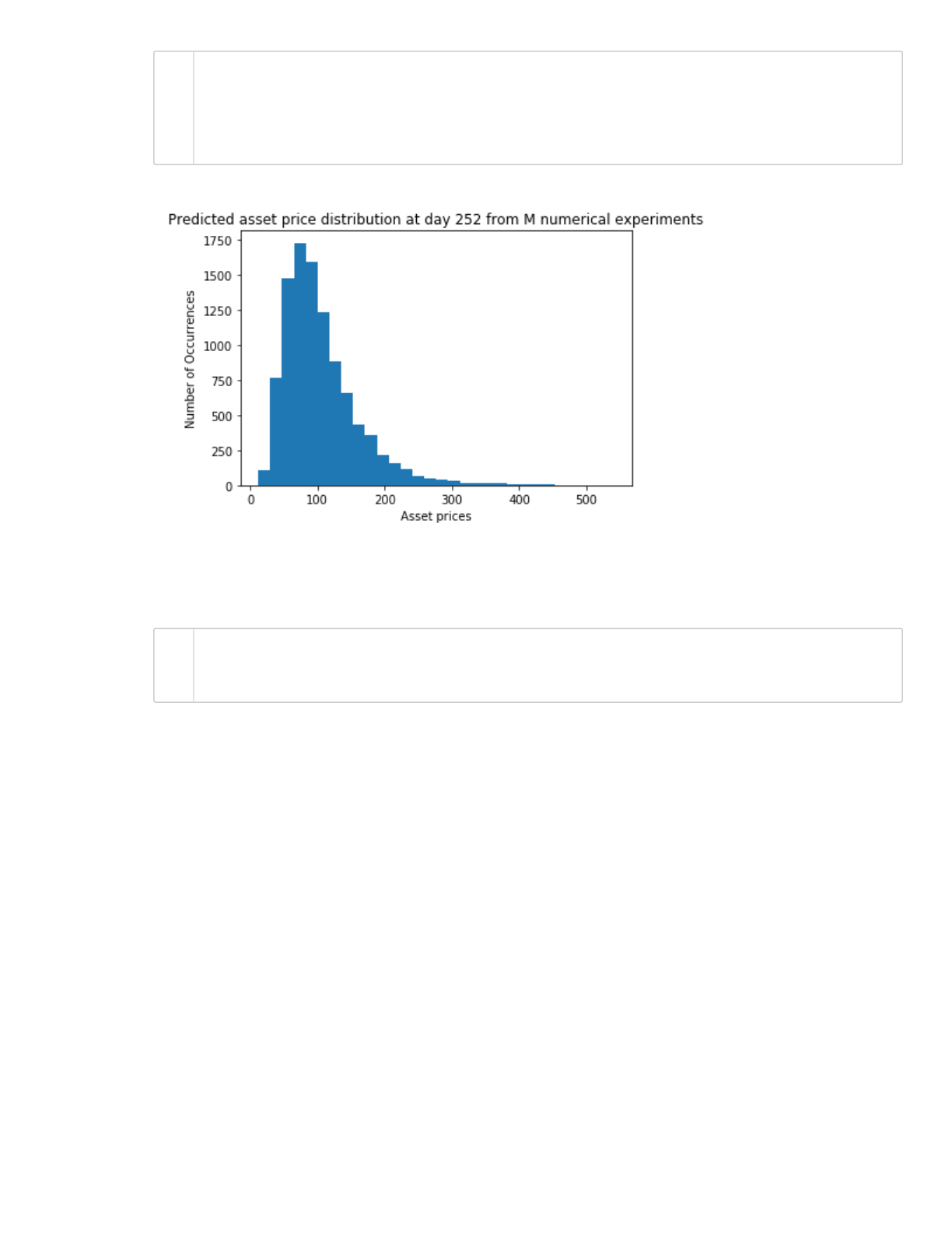
Plot the histogram of the predicted prices:
N = 252 # days
M = 10000 # number of numerical experiments
S0 = 100 # initial asset price
r = 0.05
sigma = 0.5
#clear
price_M = []
for j in range(M):
price = [S0]
for i in range(N):
price.append( St_GBM(price[-1],r,sigma,deltaT) )
price_M.append(price)
price_M = np.array(price_M).T
plt.figure()
plt.plot(price_M);
plt.title ('M numerical experiments of Black-Scholes Model');
plt.xlabel('Day');
plt.ylabel('Price');
#clear
predicted_prices = price_M[-1,:]
1
2
3
4
5
1
2
3
4
5
6
7
8
1
2
3
4
5
1
2
2/18/2020 MonteCarloMethods
localhost:8888/notebooks/GitCourseRepo/cs357-sp20/assets/demos/6-monte-carlo/MonteCarloMethods.ipynb#b)-Write-a-function-to-evaluate-the-probability-the-
…
27/36
In[56]:
Calculate the mean and standard deviation of the distribution for the stock on the last day. What do
you get?
In[57]:
Congratulations! You now have a prediction for a future price for a given stock.
Example 7) An example of a 2-d random walk
Mariastenchia was in urgent need to use the restroom. Luckly, she saw Murphy's pub open and
decided to go in for relief.
Unfortunately, Mariastenchia is not feeling very well, and due to some unknown reasons, she is
confused and dizzy, and hence not sure if she can make it to the bathroom. After a quick evaluation,
she decided that if she cannot get there in less than 100 steps, she will be in serious trouble.
Do you think she can make a successful trip to the restroom? Let's help her estimating her odds.
Out[56]:
Text(0, 0.5, 'Number of Occurrences')
104.79243653779879 55.96051966865237
plt.figure()
plt.hist(predicted_prices,30);
plt.title('Predicted asset price distribution at day 252 from M numerica
plt.xlabel('Asset prices')
plt.ylabel('Number of Occurrences')
#clear
print( predicted_prices.mean(), predicted_prices.std() )
1
2
3
4
5
1
2
3

2/18/2020 MonteCarloMethods
localhost:8888/notebooks/GitCourseRepo/cs357-sp20/assets/demos/6-monte-carlo/MonteCarloMethods.ipynb#b)-Write-a-function-to-evaluate-the-probability-the-
…
28/36
The helper function below plots the floor plan.
In[58]:
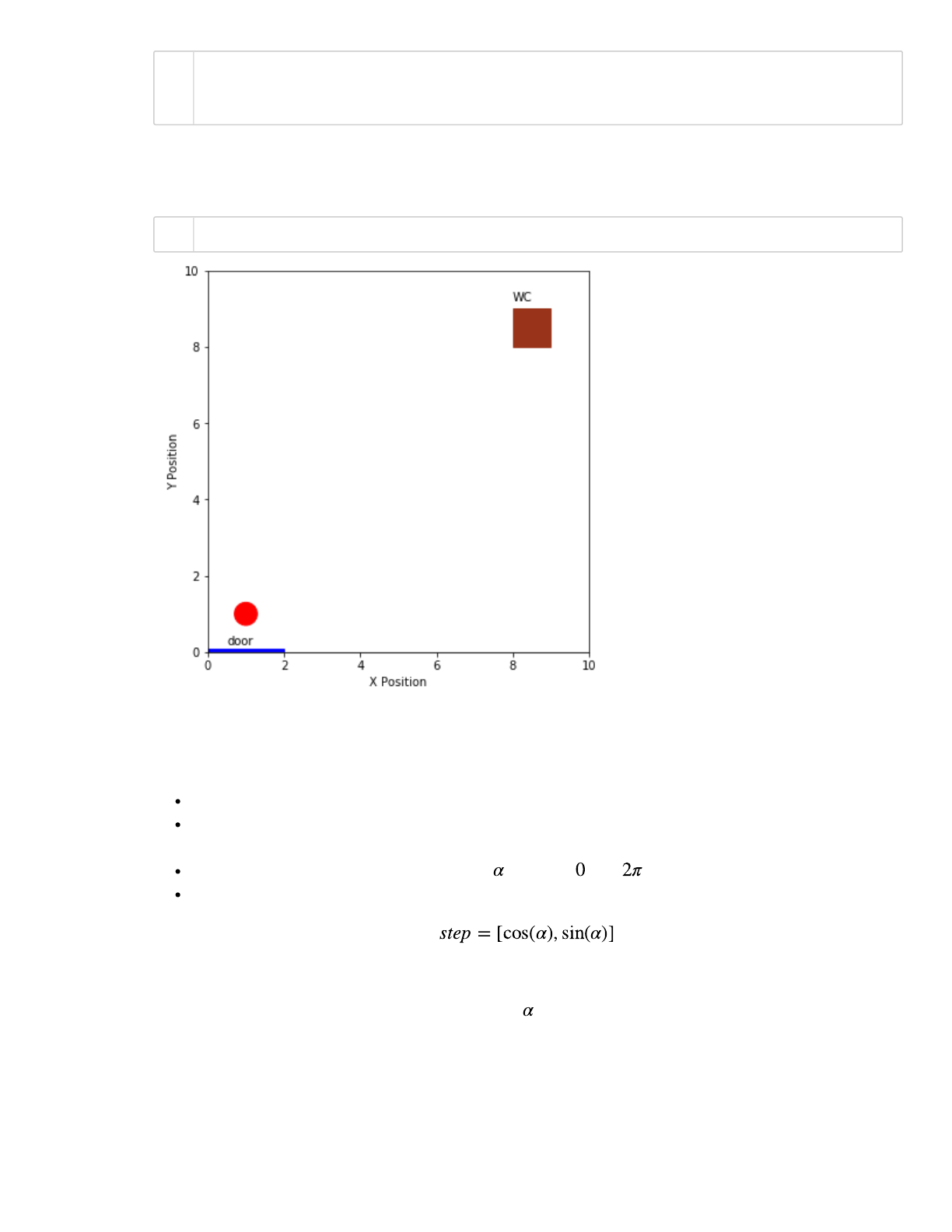
Let's take a look at the floor plan of Murphy's pub
We will simplify the floor plan with a square domain of size room_size = 10. The bottom left
corner of the room will be used as the origin, i.e. the position (x,y) = (0,0).
The bathroom location is indicated by a square, with the left bottom corner located at (8,8) and
dimension h = 1. These quantities are stored as a tuple bathroom = (8,8,1).
The street door is located at the bottom half, indicated by the blue line. Mariastenchia initial position
is given by initial_position = (1,1), marked with a red half-dot.
# Helper function to draw the floor plan
# You should not modify anything here
def draw_murphy(wc,person,room_size):
fig = plt.figure(figsize=(6,6))
ax = fig.add_subplot(111)
plt.xlim(0,room_size)
plt.ylim(0,room_size)
plt.xlabel("X Position")
plt.ylabel("Y Position");
ax.set_aspect('equal')
rect = plt.Rectangle(wc[:2], wc[-1], wc[-1], color=(0.6,0.2,0.1) )
ax.add_patch(rect)
plt.text(wc[0],wc[1]+wc[2]+0.2,"WC")
rect = plt.Rectangle((0,0),2,0.1, color=(0,0,1) )
ax.add_patch(rect)
plt.text(0.5,0.2,"door")
circle = plt.Circle(person[:2], 0.3, color=(1,0,0))
ax.add_patch(circle)
1
2
3
4
5
6
7
8
9
10
11
12
13
14
15
16
17
18
19
20
21
2/18/2020 MonteCarloMethods
localhost:8888/notebooks/GitCourseRepo/cs357-sp20/assets/demos/6-monte-carlo/MonteCarloMethods.ipynb#b)-Write-a-function-to-evaluate-the-probability-the-
…
29/36
In[59]:
We will simplify Mariastenchia's challenge and remove all the tables and the bar area inside
Murphy's. Here is how the room looks like in our simplified floor plan:
In[60]:
How are we going to model Mariastenchia's walk?
Since Mariastenchia is dizzy and confused, we will model her steps as a random walk.
Each step will be modeled by a magnitude and direction in a 2d plane. We will assume the
magnitude as 1.
The direction is given by a random angle between and .
Combining the angle and magnitude, her step is defined as:
Write the function random_step that takes as argument the current position, and returns the new
position based on a random step with orientation .
room_size = 10
bathroom = (8,8,1)
initial_position = (1,1)
draw_murphy(bathroom,initial_position,room_size)
1
2
3
1

2/18/2020 MonteCarloMethods
localhost:8888/notebooks/GitCourseRepo/cs357-sp20/assets/demos/6-monte-carlo/MonteCarloMethods.ipynb#b)-Write-a-function-to-evaluate-the-probability-the-
…
30/36
def random_step(current_position):
# current_position is a list: [x,y]
# x is the position along x-direction, y is the position along y
-direction
# new_position is also a list: [xnew,ynew]
# Write some code here
return new_position
In[61]:
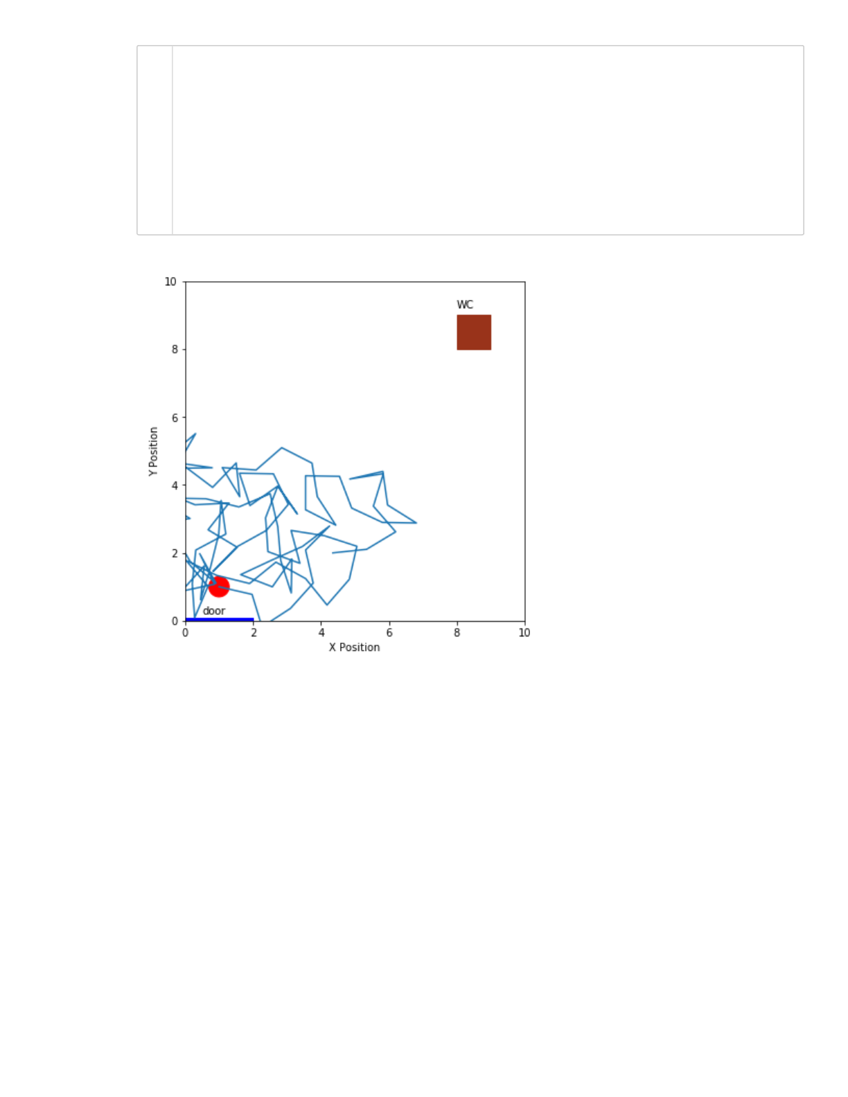
Let's make Mariastenchia give her 100 steps, using the function random_step. Complete the code
snippet below, and plot her path from the door (given by the variable initial_position above) to
her final location. Did she reach the bathroom?
Code snippet A
position = #create a list to store all the 100 positions
# Write code to simulate Mariastenchia 100 steps
draw_murphy(bathroom,initial_position,room_size)
x,y = zip(*position)
plt.plot(x,y)
#clear
def random_step(current_position):
theta = random.randint(0,360)
new_position = current_position.copy()
new_position[0] += np.cos(theta*np.pi/180)
new_position[1] += np.sin(theta*np.pi/180)
return(new_position)
1
2
3
4
5
6
7
2/18/2020 MonteCarloMethods
localhost:8888/notebooks/GitCourseRepo/cs357-sp20/assets/demos/6-monte-carlo/MonteCarloMethods.ipynb#b)-Write-a-function-to-evaluate-the-probability-the-
…
31/36
In[62]:
You probably noticed Mariastenchia hitting walls, or even walking through them! Let's make sure we
Out[62]:
[<matplotlib.lines.Line2D at 0x13947a5c0>]
#clear
N = 100
position = [list(initial_position)]
for i in range(N-1):
new_position = random_step(position[-1])
position.append(new_position)
draw_murphy(bathroom,initial_position,room_size)
x,y = zip(*position)
plt.plot(x,y)
1
2
3
4
5
6
7
8
9
10

2/18/2020 MonteCarloMethods
localhost:8888/notebooks/GitCourseRepo/cs357-sp20/assets/demos/6-monte-carlo/MonteCarloMethods.ipynb#b)-Write-a-function-to-evaluate-the-probability-the-
…
32/36
p y g , g g
impose this constraints to the random walk, so we can get some feasible solution. Here are the rules
for Mariastenchia's walk:
If Mariastenchia runs into a wall, the simulation stops, and we call it a "failure" (ops!)
If the sequence of steps takes Mariastenchia to the restroom, the simulation stops, and we call
it a success (yay!).
To simplify the problem, the "restroom" does not have a door, and Mariastenchia can "enter" the
square through any of its sides.
Mariastenchia needs to reach the restroom in less than 100 steps, otherwise the simulation
stops (at this point, it is a little too late for her...). This is also called a failure.
Write the function check_rules that checks if the new_position is a valid one, according to the
rules above. The function should return 0 if the new_position is a valid step (still inside Murphy's
and searching for the restroom), 1 if new_position is inside the restroom (sucess), and -1 if
new_position is a failure (Mariastenchia became a super woman and crossed a wall)
def check_rules(room_size,wc,current_position):
# write some code here
# return 0, 1 or -1
In[63]:
In[64]:
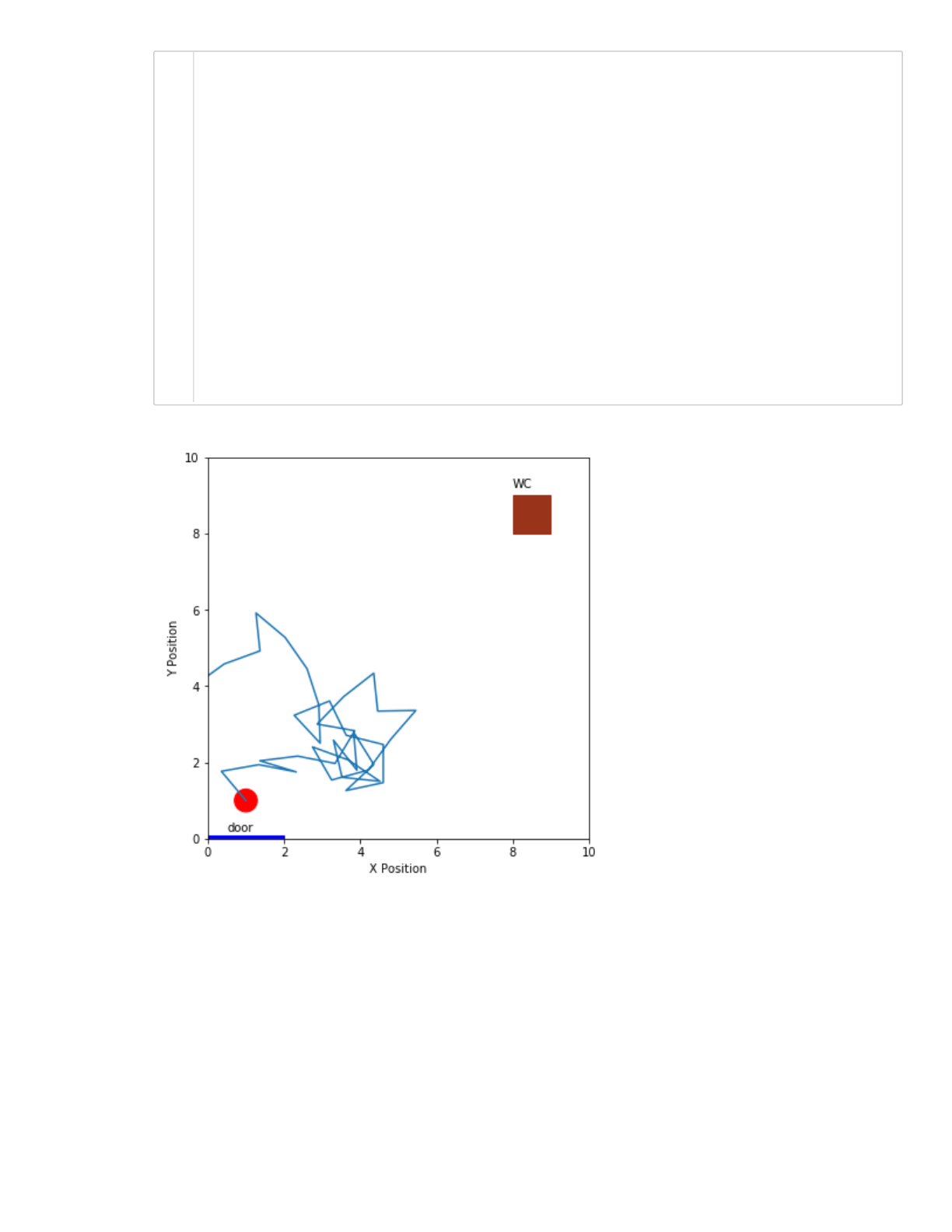
Modify your code snippet A above, so that for every step, you check for the constraints using
check_rules. Instead of giving all the 100 steps, you should stop earlier in case she reaches the
restroom (check_rules == 1) or she hits a wall ( check_rules == -1)
Code snippet B
-1
0
1
#clear
def check_rules(room_size,wc,current_position):
x,y,h = wc
# Checking if inside the room:
if ( (current_position[0] > 0) & (current_position[0] < room_size) &
# Checking if found the restroom
if ( (current_position[0] > x) & (current_position[0] < x + h) &
return 1
else:
return 0
else:
return (-1)
# Try your function check_rules with the following conditions:
print(check_rules(room_size,bathroom,[-1,0]))
print(check_rules(room_size,bathroom,[5,5]))
print(check_rules(room_size,bathroom,[8.5,8.5]))
1
2
3
4
5
6
7
8
9
10
11
12
1
2
3
4
2/18/2020 MonteCarloMethods
localhost:8888/notebooks/GitCourseRepo/cs357-sp20/assets/demos/6-monte-carlo/MonteCarloMethods.ipynb#b)-Write-a-function-to-evaluate-the-probability-the-
…
33/36
In[65]:
It looks like this random walk does not give her much of a chance to get to the restroom. She may
need more steps, or we can modify her walk to be a little less random. All you need to do is to
modify your function random_step. What about we make her move forwards (in the positive
direction of y) with a 70% probability (meaning she would move backwards with 30% probability).
Out[65]:
[<matplotlib.lines.Line2D at 0x139ab1fd0>]
#clear
position = [list(initial_position)]
for i in range(N):
new_position = random_step(position[-1])
position.append(new_position)
result = check_rules(room_size,bathroom,new_position)
if result == 1:
# found the wc
break
elif result == -1:
# hit a wall
break
draw_murphy(bathroom,initial_position,room_size)
x,y = zip(*position)
plt.plot(x,y)
1
2
3
4
5
6
7
8
9
10
11
12
13
14
15
16
17

2/18/2020 MonteCarloMethods
localhost:8888/notebooks/GitCourseRepo/cs357-sp20/assets/demos/6-monte-carlo/MonteCarloMethods.ipynb#b)-Write-a-function-to-evaluate-the-probability-the-
…
34/36
In[66]:
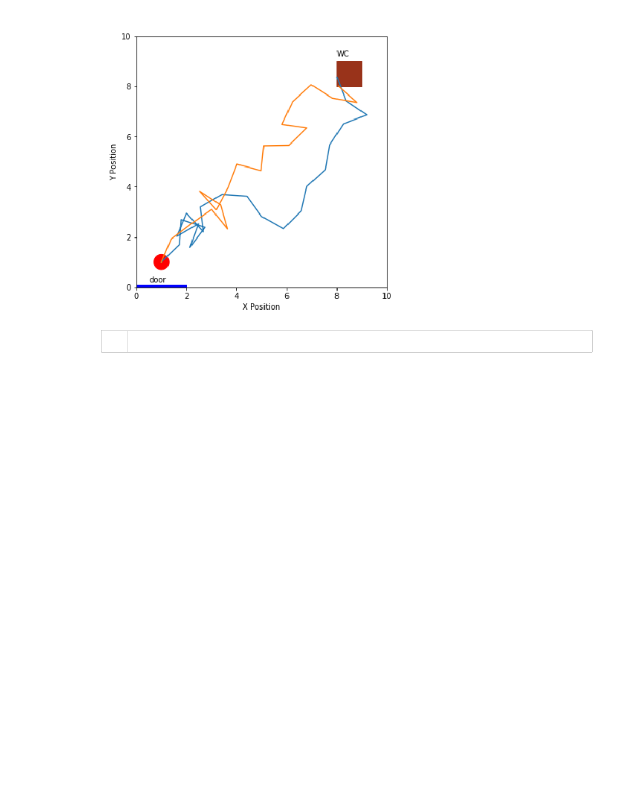
Let's estimate the probability Mariastenchia reaches the restroom:
You should now run many simulations (one attempt to reach the restroom), and tally how many
attempts are successful. The probability to reach the bathroom is n_success/M.
#clear
def random_step_prob(current_position):
if random.random() > 0.3:
theta = random.randint(0,180)
else:
theta = random.randint(180,360)
new_position = current_position.copy()
new_position[0] += np.sin(theta*np.pi/180)
new_position[1] += np.cos(theta*np.pi/180)
return(new_position)
1
2
3
4
5
6
7
8
9
10

2/18/2020 MonteCarloMethods
localhost:8888/notebooks/GitCourseRepo/cs357-sp20/assets/demos/6-monte-carlo/MonteCarloMethods.ipynb#b)-Write-a-function-to-evaluate-the-probability-the-
…
35/36
In[67]:
probability is 0.01797
#clear
success = 0
track_paths = []
M = 100000
N = 300
for i in range(M):
position = [list(initial_position)]
for j in range(N):
new_position = random_step_prob(position[-1])
position.append(new_position)
result = check_rules(room_size,bathroom,new_position)
if result == 1:
# found the wc
success += 1
break
elif result == -1:
# hit a wall
break
if ((result == 1) & (not i%(M/100))):
track_paths.append(position)
draw_murphy(bathroom,initial_position,room_size)
for l in range(len(track_paths)):
x,y = zip(*track_paths[l])
plt.plot(x,y)
print("probability is ", success/M)
1
2
3
4
5
6
7
8
9
10
11
12
13
14
15
16
17
18
19
20
21
22
23
24
25
26
27
28
29
30
31
32
33
2/18/2020 MonteCarloMethods
localhost:8888/notebooks/GitCourseRepo/cs357-sp20/assets/demos/6-monte-carlo/MonteCarloMethods.ipynb#b)-Write-a-function-to-evaluate-the-probability-the-
…
36/36
In[]:
1
