
Adding the latency period to a
muscle contraction model
coupled to a membrane action
potential model
Nadia Roberta Chaves Kappaun
1
,
2
,
Ana Beatriz Nogueira Rubião Graça
1
,
Gabriel Benazzi Lavinas Gonçalves
1
, Rodrigo Weber dos Santos
1
,
Sara Del Vecchio
3
and Flávia Souza Bastos
1
*
1
Graduate Program in Computational Modeling, Federal University of Juiz de Fora, Juiz de Fora, Brazil,
2
National Cancer Institute, Rio de Janeiro, Brazil,
3
Federal Institute of Education, Science and Technolog y
of the Southeast of Minas Gerais, Juiz de Fora, Brazil
Introduction: Skeletal muscle is responsible for multiple functions for maintaining
energy homeostasis and daily activities. Muscle contraction is activated by nerve
signals, causing calcium release and interaction with myofibrils. It is important to
understand muscle behavior and its impact on medical conditions, like in the
presence of some diseases and their treatment, such as cancer, which can affect
muscle architecture, leading to deficits in its function. For instance, it is known that
radiotherapy and chemotherapy also have effects on healthy tissues, leading to a
reduction in the rate of force development and the atrophy of muscle fibers. The
main aim is to reproduce the behavior of muscle contraction using a coupled
model of force generation and the action potential of the cell membrane, inserting
the latency period observed between action potential and force generation in the
motor unit.
Methods: Mathematical models for calcium dynamics and muscle contraction are
described, incorporating the role of calcium ions and rates of reaction. An action
potential initiates muscle contraction, as described by the Hodgkin–Huxley
model. The numerical method used to solve the equations is the forward Euler
method.
Results and Discussion: The results show dynamic calcium release and force
generation, aligning with previous research results, and the time interval between
membrane excitation and force generation was accomplished. Future work
should suggest simulating more motor units at the actual scale for the
possibility of a comparison with real data collected from both healthy
individuals and those who have undergone cancer treatment.
KEYWORDS
skeletal muscle model, muscle contraction, latency period, calcium dynamics, action
potential model, finite-difference method
OPEN ACCESS
EDITED BY
Alexandre Lewalle,
King’s College London, United Kingdom
REVIEWED BY
Roberto Piersanti,
Polytechnic University of Milan, Italy
Yixuan Wu,
University of California, Davis,
United States
*CORRESPONDENCE
Flávia Souza Bastos,
RECEIVED 18 October 2023
ACCEPTED 24 November 2023
PUBLISHED 18 December 2023
CITATION
Kappaun NRC, Graça ABNR,
Lavinas Gonçalves GB,
Weber dos Santos R, Vecchio SD and
Bastos FS (2023), Adding the latency
period to a muscle contraction model
coupled to a membrane action
potential model.
Front. Phys. 11:1323542.
doi: 10.3389/fphy.2023.1323542
COPYRIGHT
© 2023 Kappaun, Graça, Lavinas
Gonçalves, Weber dos Santos, Vecchio
and Bastos. This is an open-access article
distributed under the terms of the
Creative Commons Attribution License
(CC BY). The use, distribution or
reproduction in other forums is
permitted, provided the original author(s)
and the copyright owner(s) are credited
and that the original publication in this
journal is cited, in accordance with
accepted academic practice. No use,
distribution or reproduction is permitted
which does not comply with these terms.
Frontiers in Physics frontiersin.org01
TYPE Original Research
PUBLISHED 18 December 2023
DOI 10.3389/fphy.2023.1323542
1 Introduction
Skeletal muscle is an efficient and adaptable tissue responsible
for multiple functions for maintain ing energy homeostasis and
daily act ivities [1]. It is composed of blood vessels, connective
tissues, and muscle cells known as muscle fibers. A muscle fibe r is
a long and slender cell whose primary component is the
myofibril. Myofibrils play a central role in i nitiating muscle
cell contractions due to the presence of two vit al filament
types: actin and myosin [ 2].
Muscle fibers produce force through electrical activation by the
nervous system, allowing for muscle contraction and, consequently,
motion (Peterson and Bronzino [3]). The interaction between a
nerve and a muscle fiber is known as a synapse, and the entire
process is initiated by the arrival of an action potential. A motor unit
(MU) comprises all the muscle cells controlled by a single nerve
fiber. The nerves responsible for controlling muscles are known as
motor neurons [2].
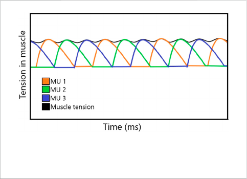
Motor units are controlled through synchronous
recruitment by the central nervous system. This type of
recruitment, as shown in Figure 1, recruits one unit at a time
to maintain constant tension and, i f necessary, recruits different
motor units simultaneously to generate greater tension in the
muscle [ 4]. Farina et al. [5] stated that recruitment begins with
the smallest muscle fibers, which typically exhibit the lowest
conduction veloc ity. The controlled a ctivation of motor unit
populations accomplishes movement, as described in [6], which
was based on th e understanding of motor unit physiology
through computational and experimental studies. However,
muscles do not develop tension immediately; instead, there is
a brief period known a s the latency period before t ension is
generated [2].
The contractile system of skeletal muscles is regulated by ions
Ca
2+
, which are stored in t he sarcoplasmic ret iculum (SR). It was
stated in [2] that the release of ions Ca
2+
into the c ytoplasm of
muscle cells is triggered by the arri valofanactionpotentialatthe
motor end plate, followed b y neur otransmitter release and uptake
bythemusclecells.WhenCa
2+
is removed from the cytoplasm,
the contraction process ceases , and the muscle returns to its
initial length. The net effect of a single action potential results in a
transient contraction of the motor unit, commonly referred to as
a twitch.
Studying skeletal muscle and its physiological functioning
can be important for understanding its behavior in medical
conditions, such as muscle fatigue [8,9], bone diseas es [10,11],
muscular damage [12], dystrophies [13], and diseases o f
treatment sequelae [14–19]. Commonly used cancer
treatments, inc luding ch emotherapy [20–22] and radiation
therapy [23], affect skeletal muscle, inducing a decr ease in the
rate of force development and loss in muscle fibers, which lea ds to
a change in muscle function and promotion of its inflammation
[17]. It was stated in [18]and[19]that can cer survivors
experience several treatment-related symptoms, muscular
weakness, and reduced mobility, thereby compromising their
quality of life. Furthermore, after pelvic radiotherapy, the
exposure of the anal canal and nerve s of the sacral plexus to
radiation may be associated with the deterioration of sphincter
function [24], and changes are observed in the composition of the
pelvic floor muscle structure, which was maintained even after
4 yea rs of treatment for prostate or colorectal cancer [25]. In
addition, functional modificationsinthepelvicfloor have been
reported, such as reduced pressures at rest and during maximum
contraction after radiotherapy, for up to 1 year after treatment
[26]. It was suggested in [23 ] that ionizing irradiation leads to a
reduction in the perimeter and contractility of muscle fibers as
well as a lower amount of skin fiber renewal. Late effects of
radiotherapy include gastrointestinal, urological, female
reproductive tract, skeletal, and vascular toxicity, secondary
malignancies, and quality-of-life issues [27–29].
Recent studies focused on the association b etween skelet al
muscle quality and the prognosis of pat ients with gynecological
cancer [14 –16,30 ]. In [15], it was shown that maintaining muscle
mass can prolong survival in cancer patients, and the work in [16]
related that visceral obesity before radiother apy and
chemotherapy has a protective effect on the prognosis of
patients with stage IVB cervic al can cer, while a low muscle
index and low visceral-to-subcutaneous adipose tissue area
ratio are associated with worse prognosis. Research studies
also identified a low pretreatment skeletal muscle index as a
prognostic factor for overall survival in patients diagnosed with
cervical or ovarian cancer [14,31]. O n the other hand, in [ 30],
datafromtheskeletalmuscleareawerereviewedtoidentify
skeletal muscle mass loss (sarcopenia) in patients with cervical,
endometrial, and ovarian cancers, appointing that the limited
literature data seem to suggest that baseline muscle indexes have
an uncertain prognostic pertinence, whereas their changes during
treatment often corre spond with chances of patient survival.
Although a novel sarcopenia measure combining quantity and
quality of muscle is i mportant to spread the basis to explain the
relationship between sarcopenia and solid tumor aftereffects
considering high-risk patients [31], there is a lack of studies
that analyze muscle changes during cancer treatments, which
might be justified by the d iscrepancy in measuremen t methods of
muscle depletion across rese arch studies [17].
The overall electrical activity of skeletal muscles can be
measured by electromyography (EMG). However, EMG signals
are diffic ult to inter pret since they are con trolled by the nervous
system and are dependent on the anatomical and physiological
properties of muscles [32]. Additionally, for breast cancer
FIGURE 1
Tension developed in each MU, resulting in a constant tension in
the muscle.
Frontiers in Physics frontiersin.org02
Kappaun et al. 10.3389/fphy.2023.1323542
patients, surgery and radiation therapies impact shoulder muscle
health throughout c hangesinmusclemorphologyand
neuromuscular function. Notwit hstanding, besides the
conflicting results, EMG amplitudes o btained during motion
activities demonst rate that the neuromuscular strategy and
control may be depe ndent on the treatment received [33].
Mathematical and computational modeling can help
investigate the characteristics of EMG signals and test their
accuracy and validity. Mathematical modeling allows the
estimation of parameters that are not directly accessible for
measurements, for example, related to the description of the
spatial and temporal recruitm ent of motor unit s [34]. Moreover,
it can help in developing tools to measure the force developed by
amuscle[35].
The objective here is to reproduce t he beha vior of muscle
contraction using a coupled model of f orce generation and the
action potential of the cell me mbrane, associated with Ca
2+
regulation, inserting the latencyperiodobservedbetweenthe
action potential in the membrane and force generation in the
motor unit.
2 Materials and methods
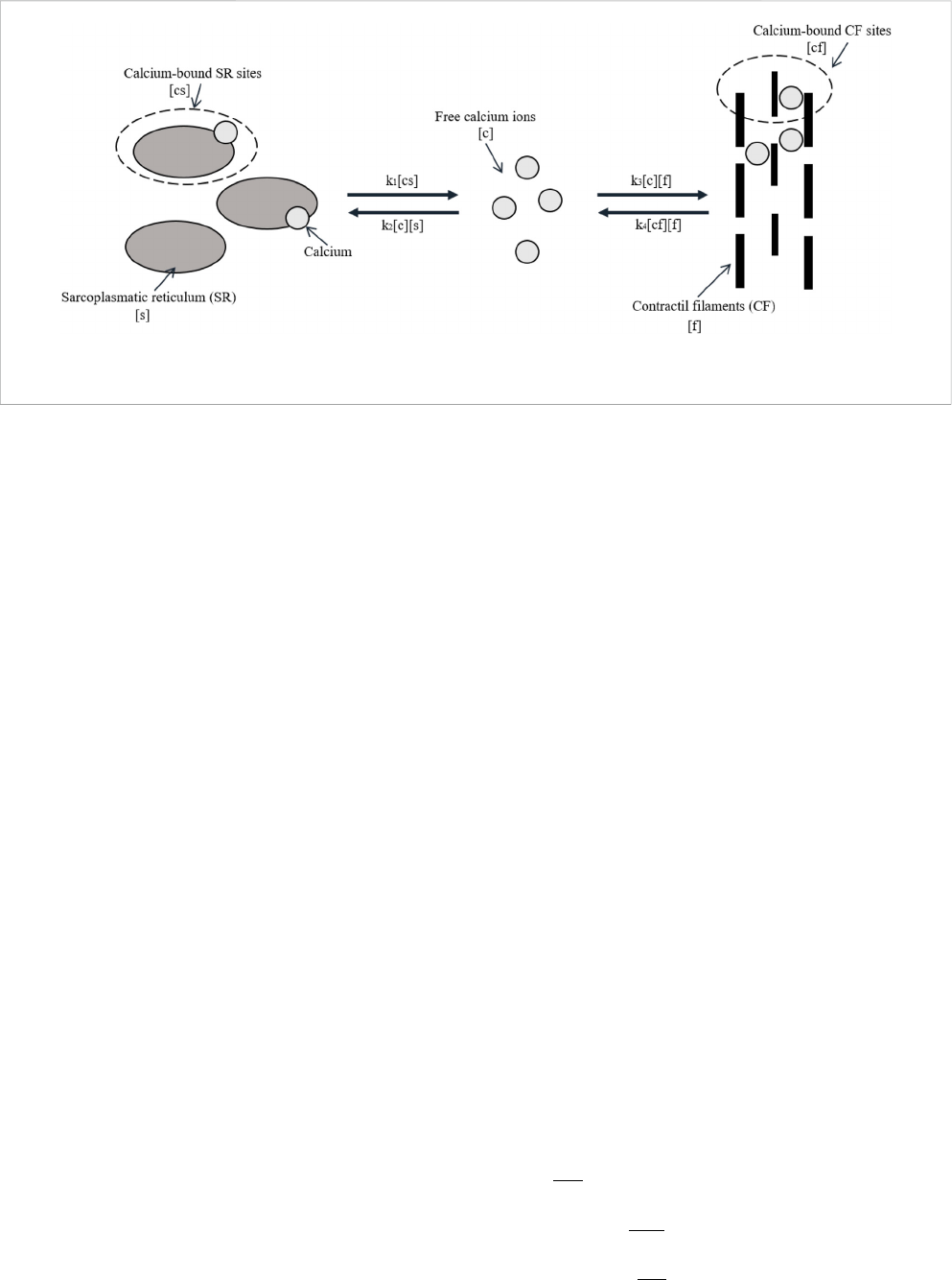
2.1 Calcium dynamics and muscle
contraction models
The mathematical model of calcium dynamics and muscle
contraction was based on the work in [36] that appears in the
work in [37]and[38], which uses simple ma ss actio n kineti cs to
describe calcium d ynamics in t he mus cle. The model is shown in
Figure 2. It describes the relationship be tween concen trations of
free calcium ions [c], unbound SR calcium binding [s], unbound
contractile filaments (CFs) calcium binding [f], calcium-bound
SR sites [cs], and calcium-bound CF sites [cf].
The rates at which reactants act are represented by parameters
k
i
. The rates k
1
and k
2
operate similar to a switch, dependent on the
value of the action potential of muscle V
m
, as shown by the following
equations:
k
1
V
m
t − T
()()
k
1
, if V
m
t − T
()
> V
min
0, otherwise
, (1)
k
2
V
m
t − T
()()
k
2
, if V
m
t − T
()
< V
min
0, otherwise
, (2)
where V
m
is the action potential in the membrane, V
min
is its
minimum value to activate the contraction process, and T is the
latency period (in ms) between the action potential in the membrane
and the onset of contraction. The inclusion of delay was
implemented by a delay-differential equation (DDE), as evaluated
in [39], which achieved dynamics similar to the original
FitzHugh–Nagumo and Hodgkin–Huxley models using a single
DDE formulation in each case.
When a muscle is activated, k
1
represents the rate constant
for the rele ase of calcium from the SR and k
2
= 0. Whe n the
muscle is not activated, k
1
=0andk
2
represent the rate constant
for the binding of calcium to the SR. Likewise, the rate of
binding of calcium-bound CF sites is proportional to the
concentration of both free calcium ions and unbound
calcium-binding sites with rate constant k
3
.Thereversible
process occurs with rate constant k
4
, a nd it is proportional
to the concentration of both bound and unbound CF sites. In
[38], it was explained that it was necessary to introduce some
cooperativity in the release of calcium so that the relaxation
process does not begin abru ptly. Although diffe rent from the
relationship of k
1
and k
2
, k
3
and k
4
can both be non-zero at the
same time. The differential equations of calcium dynamics are
as follows:
dc
[]
dt
k
1
cs
[]
− k
2
c
[]
s
[]
− k
3
c
[]
f
+ k
4
cf
f
, (3)
dcs
[]
dt
−k
1
cs
[]
+ k
2
c
[]
s
[]
, (4)
ds
[]
dt
k
1
cs
[]
− k
2
c
[]
s
[]
, (5)
FIGURE 2
Model of calcium dynamics. Adapted from McMillen, Williams, and Holmes [36] licensed Creative Commons Attribution 4.0 International.
Frontiers in Physics frontiersin.org03
Kappaun et al. 10.3389/fphy.2023.1323542
dcf
dt
k
3
c
[]
f
− k
4
cf
f
, (6)
df
dt
−k
3
c
[]
f
+ k
4
cf
f
.(7)
It is assumed the total number of calcium ions (C), SR-binding
sites (S), and filament-binding sites (F) remains constant, following
mass conservation laws:
c
[]
+ cf
+ cs
[]
C, (8)
s
[]
+ cs
[]
S, (9)
f
+ cf
F. (10)
Combining the differential equations from mass action kinetics
and mass conservation laws yields
dc
[]
dt
k
1
C − c
[]
− cf
− k
2
c
[]
S − C + c
[]
+ cf
− k
3
c
[]
F − cf
+ k
4
cf
F − cf
,
(11)
dcf
dt
k
3
c
[]
F − cf
− k
4
cf
F − cf
. (12)
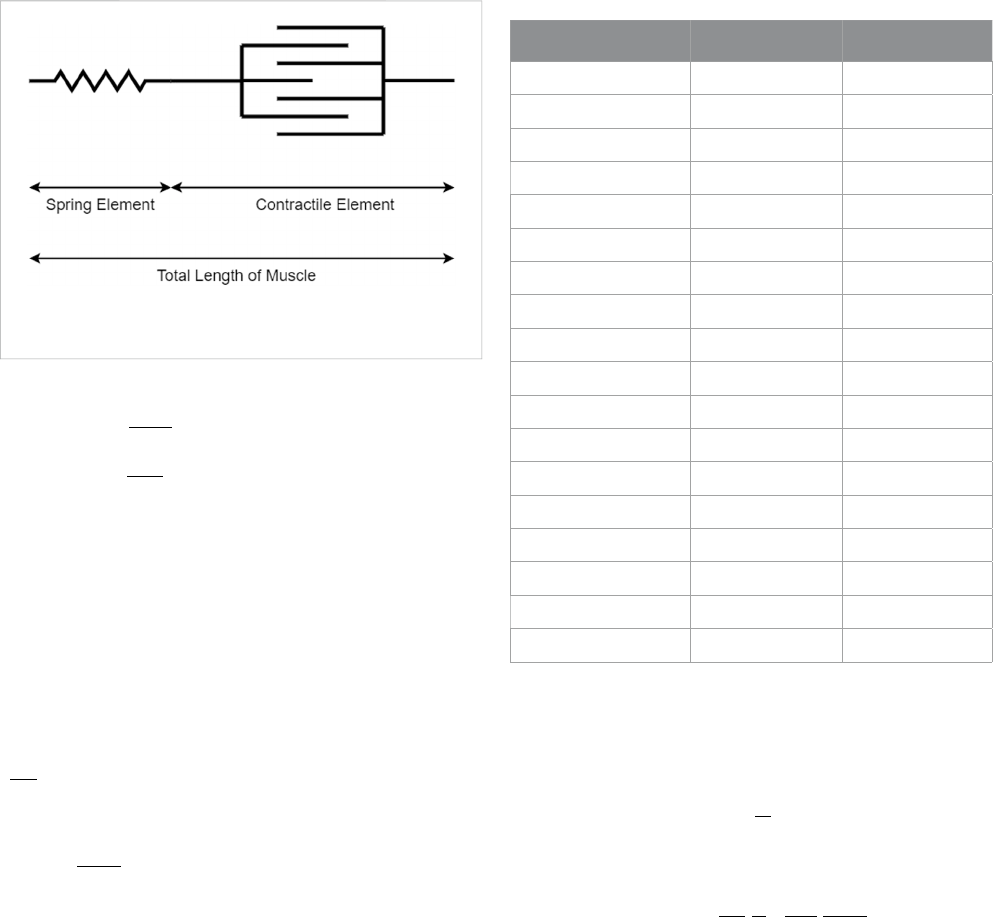
Accordingly to the work in [ 3], there are three general classes
of models for predicting muscle force: biochemical models,
constitutive models, or Hill’smodels.In[36], Hill’smodel
based on the work in [40] was used, which describes the
muscle as a contractile element in series with a linearly spring
element, as shown in Figure 3. The model says that the total
length of muscle corresponds to the length of the contractile
element l
c
plus the length of the linearly spring element l
s
:
L l
c
+ l
s
. (13)
According to Hooke’s law, the total force in a linearly elastic
body is proportional to the final length of that body minus the initial
length:
P
s
μ
s
l
s
− l
s
0
, (14)
where P
s
is the applied force, l
s
is the final length, l
s
0
is the initial
length, and the proportionality constant μ
s
is Young’s modulus, or
stiffness constant. In Hill’s model, that stiffness varies when muscle
exerts force from total relaxation.
μ
s
μ
0
+ μ
1
cf
. (15)
Combining Eq. 13 with Eq. 14 and isolating l
c
yield
l
c
L −
P
s
μ
s
+ l
s
0
. (16)
Taking the time derivative of Eq. 16 yields
v
c
Vt
()
−
dP
s
dt
1
μ
s
+
μ
1
P
s
μ
s
2
dcf
dt
, (17)
where v
c
and V(t) are the time derivatives of l
c
and L,
respectively.
Assuming that the muscle performs an isometric
contraction, its tot al length L(t) is constant, and time
derivative V(t)isnull.
As assumed in [36], the applied force on the contractile element
(P
c
) is proportional to independent multiplicative factors of its
length (l
c
) and velocity (v
c
):
P
c
P
0
λ l
c
()
α v
c
()
cf
. (18)
Furthermore, dividing Eq. 18 by P
0
provides a non-dimensional
value for P
c
, as was carried out in [38].
P
c
λ l
c
()
α v
c
()
cf
. (19)
The functions λ(l
c
)andα(v
c
) were measured in [36], which
provided a linear function for α and a quadratic function for λ as
follows:
FIGURE 3
Simplified Hill’s model for predicting muscle force.
TABLE 1 Input parameters for the action potential model.
Parameter Value Citation
k
1
(activated) 9.6 s
−1
[37]
k
2
(activated) 5.9 s
−1
[37]
k
3
65 s
−1
[37]
k
4
45 s
−1
[37]
k
5
100 s
−1
[37]
C 15 -
S 15 -
F 15 -
L 2.7 mm [37]
μ
0
1[38]
μ
1
23 [38]
λ
2
−20 [38]
l
c0
2.6 mm [37]
α
max
1.8 [37]
α
p
1.33 s/mm [37]
α
m
0.4 s/mm [37]
V
min
−20 mV -
T 10 ms [2]
Frontiers in Physics frontiersin.org04
Kappaun et al. 10.3389/fphy.2023.1323542
α v
c
()
1 +
α
m
v
c
if v
c
< 0
α
p
v
c
if v
c
≥ 0
, (20)
λ l
c
()
1 + λ
2
l
c
− l
c0
()
2
. (21)
These functions are restricted such that 0 ≤ α(v
c
) ≤ α
max
and
0 ≤ λ(l
c
) ≤ 1. According to [3], when muscle performs concentric
contractions, i.e., the shortening of fiber muscle o ccurs, the
relationship between force and velocity is nearly hyperbolic
and r elatively lower than when it performs eccentric
contractions (lengthening of fiber muscle). This fact reflects
α
p
> α
m
> 0.
In a steady state, P
s
and P
c
must be equal. So, the transfer of force
from the contractile element to the spring element was modeled by
simple linear kinetics:
dP
s
dt
k
5
P
c
− P
s
()
, (22)
where k
5
is a selected parameter to approximate P
c
to P
s
.
To prevent instability, Eq. 17 was combined with Eq. 19 and Eq. 20:
P
c
λ 1 −
dP
s
dt
α
μ
s
+
αμ
1
P
s
μ
s
2
dcf
dt
cf
, (23)
α v
c
()
α
m
if v
c
< 0
α
p
otherwise.
. (24)
Finally, Eq. 23 was combined with Eq. 22, and isolating the time
derivative
dP
dt
, the model of muscle force was obtained:
dP
s
dt
λ cf
1 +
αμ
1
μ
2
s
dcf
[]
dt
− P
s
1
k
5
+
λα cf
[]
μ
s
. (25)
The constants used for calcium dynamics and muscle
contraction models are given in Table 1. The value of V
min
was
arbitrarily chosen by the authors to represent a minimum threshold
that must be reached for the contraction to actually occur. In the
future, it is possible to compare it with real data to adjust this
parameter. Although the model used here shares its foundation with
the model in [36], it introduces a previously unaccounted latency
period (T). As explained in [2], this latency period represents the
delay between the arrival of the action potential and the release of
Ca
+2
in the muscle cell, typically averaging between 3 and 10 ms.
Thus, the value of T was derived from the established literature.
TABLE 2 Initial conditions for each variable.
Variable Value Citation
c 0-
cf 0-
P 0 N -
V
m
−70 mV [45]
m 0.05 [42]
n 0.3 [42]
h 0.6 [42]
FIGURE 4
In the first part, the current applied to the Hodgkin–Huxley model is indicated in red, representing the nervous system command to the cell. In the
middle, the action potential curve in the cell membrane is denoted in blue, derived from the Hodgkin–Huxley model. In the lower part, indicated in green,
the force generation curve in the motor unit temporally shifted due to the latency period.
Frontiers in Physics frontiersin.org05
Kappaun et al. 10.3389/fphy.2023.1323542
2.2 Action potential model
The contraction in a motor unit begins with an action potential
reaching the motor end plate and neurotransmitters being released in
the synaptic cleft. This causes Ca
2+
to be released into the cytoplasm of
themusclecell.In[36]and[38], a high-frequency sequence of
individual stimuli, called tetanic stimulus [38], was used, while in
[37], stimuli were created based on square and exponential
functions to represent tetanic stimulus and individual electric impulse.
Here, the stimulus in the cell membrane that activates the
calcium dynamic is the action potential from the model
described by [41], explained in the Appendices. The
Hodgkin–Huxley model was chosen due to its accurate
representation of the action potential, as well as being a simpler
model (with only four differential equations) compared to more
recent ones. Considering the potential for simulating multiple motor
units, larger models become computationally expensive. The
FitzHugh–Nagumo model was also assessed for having only two
equations; however, its representation is less faithful than that of the
Hodgkin–Huxley model [42]. Moreover, many recent studies were
based on the formalism of the Hodgkin–Huxley model, while many
others employ an even simpler formulation based on a transfer
function, as indicated in [43]. As shown in [37], the stimulus is
responsible for changing the rates k
1
and k
2
.
2.3 Numerical method
The numerical method applied to solve Eqs 11, 12, 25, A1–A–A4
was Euler’s method, or forward Euler, which replaces the derivative
term by the approximation presented in the following equation [44]:
dU
dt
U
i+1
− U
i
k
, (26)
where U is the variable of interest, k is the discretization time step,
and i indicates which time step the variable U is in. This way, it was
possible to approximate variable U in time i + 1, starting from the
time t = 0, in which the state of the variables is known. So, starting
with a relaxed muscle, the membrane is at rest (without an action
potential), all calcium is in the SR, and, consequently, there is no
force developed. Thus, Table 2 shows the initial conditions used in
this paper. The conditions were chosen based on the idea that there
is no free calcium or calcium bound to filaments initially, and the cell
membrane is at rest. The value of V
m
was chosen according to the
work in [45] and the variables m, n, and h according to the work
in [42].
Compared to the backward Euler and Crank–Nicolson
model, it is faster, which is gr eat for optimizing time
simulations. The system of e quations was solved using an
algorithm implemented in Python with k = 0.001, a nd t heir
exploitation about how it was implemented is presented in the
following equations.
The ODE refers to free calcium ions:
c
i+1
c
i
+ kk
1
C − c
i
− cf
i
− k
2
c
i
S − C + c
i
+ cf
i
− k
3
c
i
F − cf
i
]. (27)
The ODE refers to calcium-bound CF sites:
cf
i+1
cf
i
+ kk
3
cf
i
F − cf
i
− k
4
cf
i
F − cf
i
.
(28)
FIGURE 5
Curves representing the dynamics of calcium release and reuptake by the SR, the presence of free calcium, and calcium bound to filaments during
the contraction process initiated by the action potential of the membrane.
Frontiers in Physics frontiersin.org06
Kappaun et al. 10.3389/fphy.2023.1323542
The ODE refers to the force developed by the muscle:
P
i+1
s
P
i
s
+ k
λ cf
i
1 +
αμ
1
P
i
s
μ
2
s
dcf
i
[]
dt
− P
i
s
1
k
5
+
λα cf
i
[]
μ
s
⎡
⎢
⎢
⎢
⎢
⎢
⎢
⎢
⎢
⎢
⎢
⎣
⎤
⎥
⎥
⎥
⎥
⎥
⎥
⎥
⎥
⎥
⎥
⎦
. (29)
The ODE refers to an action potential in the membrane:
V
i+1
m
V
i
m
+ k
I
i
app
− I
i
Na
− I
i
K
− I
i
L
C
m
, (30)
where
I
i+1
Na
g
Na
m
3
h
i
V
i
m
− V
Na
, (31)
I
i+1
K
g
K
n
4
h
i
V
i
m
− V
K
, (32)
I
i+1
L
g
L
V
i
m
− V
L
. (33)
The ODE refers to auxiliary variables:
n
i+1
n
i
+ k α
n
1 − n
i
− β
n
n
i
, (34)
m
i+1
m
i
+ k α
m
1 − m
i
− β
m
m
i
, (35)
h
i+1
h
i
+ k α
h
1 − h
i
− β
h
h
i
. (36)
3 Results
The contraction process begins with a command from the nervous
system, represented here by applied current I
app
,inthefirst part of
Figure 4. When the stimulus is large enough to generate the action
potential, calcium is released, leading to the contraction of the motor unit.
As shown in blue in Figure 4, where current I
app
has two
consecutive stimuli before 25 ms, the Hodgkin–Huxley model has
a refractory period that prevents another action potential from
occurring while one was already being developed. Consequently,
there was no force generation due to this second current stimulus.
However, stimuli applied after the refractory period generate an
action potential and, after the latency period, force in the motor unit
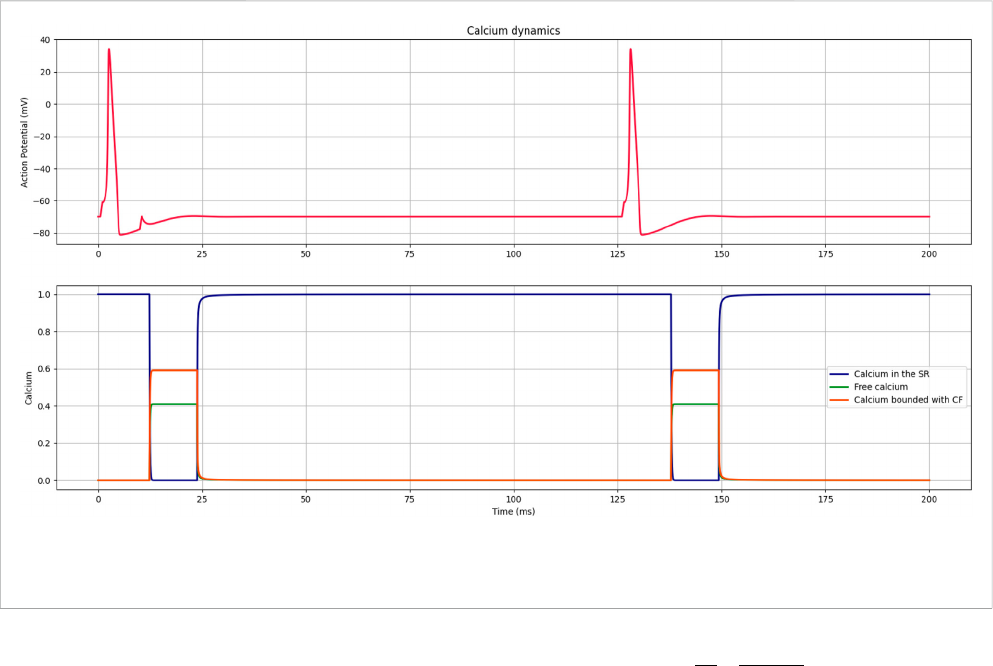
once again. Since it was set that calcium would be released starting at
a value of −20 mV, the 10-ms latency period was observed from this
point. The selection of different values for V
min
would cause the
contraction to start earlier or later, depending on the value. Here, the
value was arbitrary to represent the threshold of the muscle cell.
Figure 5 illustrates the dynamic initiated by an action potential;
first, all the calcium ions are stored in the SR, and once the potential
is generated, they are released and bind to the filaments. After some
time, the process is reversed, and all the calcium returns to SR.
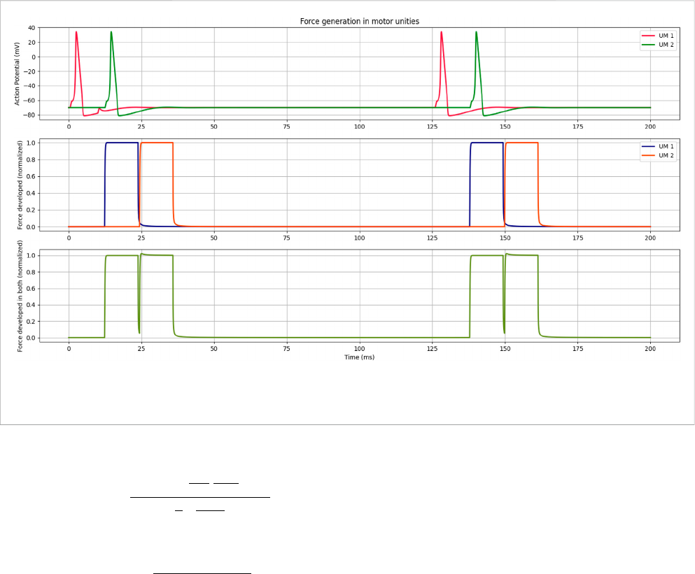
Finally, Figure 6 shows that a muscle stimulus was simulated
using two motor units to verify the total tension generated in the
muscle. It can be considered that when a high load is demanded in
major time, lots of motor units are stimulated, resulting in a higher
or longer-lasting tension developed in the muscle.
4 Discussion
A simulation coupling the Hodgkin–Huxley action potential
model to the models demonstrated in [36], [38], and [37] was
presented, adding the latency period between the stimulus and
muscle contraction to approximate the model to the real
behavior of the muscle. Although the Hodgkin–Huxley model is
relatively old, it remains a significant global reference and is
integrated into numerous research studies across the vast field of
FIGURE 6
The first part shows the action potential curves of two different motor units being stimulated. The second part shows the forces developed in both.
The third part shows the combined force of both, representing how it would be in a muscle.
Frontiers in Physics frontiersin.org07
Kappaun et al. 10.3389/fphy.2023.1323542
the electrophysiology community. Despite its use, certain biological
processes such as the activation of ion channels in the SR by the
entry of calcium for subsequent release were simpli fied by delay T
because that model does not include those processes.
The control over the rates was also different from that shown in
[37] because here, the Hodgkin–Huxley model was used to
determine the nervous stimulus associated with the release and
resorption of calcium by the SR. Therefore, the Hodgkin–Huxley
model introduced the dynamics of the sodium and potassium ions as
electrical current components, along with the calcium dynamics in
the model, which is an important component of the skeletal muscle
contraction behavior [46].
The focus of this study was on muscle behavior, simulating
reduced-size motor units. Nevertheless, it paves the way to associate
and distinguish the influence of electrical stimuli and calcium ion
dynamics on healthy muscle contraction. The question remains as to
whether alterations in muscle contraction dynamics during certain
illnesses are attributed to changes in electrical conduction or disruptions
in calcium dynamics. Hence, future efforts should involve comparing
results obtained from full-sized scenarios with a higher number of
motor units, as well as incorporating data collected from both healthy
individuals and those who have undergone cancer treatment.
Data availability statement
The original contributions presented in the study are included in
the article/Supplementary Material; further inquiries can be directed
to the corresponding author.
Author contributions
NK, AG, GL, RW, SV, and FB: writing–original draft. AG and
GL: Software.
Funding
The authors declare financial support was received for the research,
authorship, and/or publication of this article. This work was supported
by the Brazilian research funding agencies FAPEMIG, CAPES, CNPq,
and UFJF. CAPES - Processo 88881.708850/2022-0.
Conflict of interest
The authors declare that the research was conducted in the
absence of any commercial or financial relationships that could be
construed as a potential conflict of interest.
Publisher’s note
All claims expressed in this article are solely those of the authors
and do not necessarily represent those of their affiliated
organizations, or those of the publisher, the editors, and the
reviewers. Any product that may be evaluated in this article, or
claim that may be made by its manufacturer, is not guaranteed or
endorsed by the publisher.
References
1. Li F, Periasamy M. Skeletal muscle inefficiency protects against obesity. Nat Metab
(2019) 1:849–50. doi:10.1038/s42255-019-0116-x
2. Ethier CR, Simmons CA. Introductory biomechanics: from cells to organisms.
Cambridge: Cambridge University Press (2007).
3. Peterson DR, Bronzino JD. Biomechanics: principles and applications. Florida,
United States: CRC Press (2007).
4. Lynch CL. Closed-loop control of electrically stimulated skeletal muscle contractions.
Toronto, Canada: University of Toronto (2011).
5. Farina D, Fosci M, Merletti R. Motor unit recruitment strategies investigated by
surface emg variables. J Appl Physiol (2002) 92:235–47. doi:10.1152/jappl.2002.92.1.235
6. Heckman C, Enoka RM. Motor unit. Compr Physiol (2012) 2629–82. doi:10.1002/
cphy.c100087
7. Baker LL, Parker K. Neuromuscular electrical stimulation of the muscles
surrounding the shoulder. Phys Ther (1986) 66:1930– 7. doi:10.1093/ptj/66.12.1930
8. Chaparro-Cárdenas SL, Castillo-Castañeda E, Lozano-Guzmán AA, Zequera M,
Gallegos-Torres RM, Ramirez-Bautista JA. Characterization of muscle fatigue in the
lower limb by semg and angular position using the wfd protocol. Biocybernetics Biomed
Eng (2021) 41:933–43. doi:10.1016/j.bbe.2021. 06.003
9. Cavalcanti Garcia MA, Magalhães J, Imbiriba L. Temporal behavior of motor units
action potential velocity under muscle fatigue conditions. Revista Brasileira de Medicina
do Esporte (2004) 10:299–303. doi:10.1590/S1517-86922004000400007
10. Moretti A, Iolascon G. Sclerostin: clinical insights in muscle–bone crosstalk. JInt
Med Res (2023) 51. doi:10.1177/03000605231193293
11. Ferrucci L, Baroni M, Ranchelli A, Lauretani F, Maggio M, Mecocci P, et al.
Interaction between bone and muscle in older persons with mobility limitations. Curr
Pharm Des (2014) 20:3178–97. doi:10.2174/13816128113196660690
12. Stožer A, Vodopivc P, Križančić Bombek L. Pathophysiology of exercise-induced
muscle damage and its structural, functional, metabolic, and clinical consequences.
Physiol Res (2020) 565–98. doi:10.33549/physiolres.934371
13. Allen DG. Skeletal muscle function: role of ionic changes in fatigue, damage and
disease. Clin Exp Pharmacol Physiol (2004) 31:485–93. doi:10.1111/j.1440-1681.2004.
04032.x
14. Aichi M, Hasegawa S, Kurita Y, Shinoda S, Kato S, Mizushima T, et al. Low skeletal
muscle mass predicts poor prognosis for patients with stage iii cervical cancer on
concurrent chemoradiotherapy. Nutrition (2023) 109:111966. doi:10.1016/j.nut.2022.
111966
15. Abe A, Yuasa M, Imai Y, Kagawa T, Mineda A, Nishimura M, et al. Extreme
leanness, lower skeletal muscle quality, and loss of muscle mass during treatment are
predictors of poor prognosis in cervical cancer treated with concurrent chemoradiation
therapy. Int J Clin Oncol (2022) 27:983–91. doi:10.1007/s10147-022-02140-w
16. Ji C, Liu S, Wang C, Chen J, Wang J, Zhang X, et al. Relationship between
visceral obesity and prognosis in patients with stage ivb cervical cancer receiving
radiotherapy and chemotherapy. Cancer Pathogenesis Th er (202 3). d oi:10.1 016/j.
cpt.2023 .09.0 02
17. Deng Y, Zhao L, Huang X, Zeng Y, Xiong Z, Zuo M. Contribution of skeletal
muscle to cancer immunotherapy: a focus on muscle function, inflammation, and
microbiota. Nutrition (2023) 105:111829. doi:10.1016/j.nut.2022.111829
18. Schneider CM, Hsieh CC, Sprod LK, Carter SD, Hayward R. Cancer treatment-
induced alterations in muscular fitness and quality of life: the role of exercise training.
Ann Oncol (2007) 18:1957–62. doi:10.1093/annonc/mdm364
19. Kirchheiner K, Pötter R, T anderup K, Lindeg aard JC, Haie-Mede r C,
Petrič P, et al. Health-related quality of life in locally advanced cervical
cancer patients afte r definitive chemoradiation therapy including image
guided adaptive brachytherapy: an analysis from the embrace study. In t
J Radiat Oncology*Biology*Physics (2016) 94:1088–98. doi:10.1016/j.ijrobp.
2015.12.363
20. Buffart LM, Sweegers MG, de Ruijter CJ, Konings IR, Verheul HMW, van
Zweeden AA, et al. Muscle contractile properties of cancer patients receiving
chemotherapy: assessment of feasibility and exercise effects. Scand J Med Sci Sports
(2020) 30:1918–29. doi:10.1111/sms.13758
Frontiers in Physics frontiersin.org08
Kappaun et al. 10.3389/fphy.2023.1323542
21. Visovsky C. Muscle strength, body composition, and physical activity in women
receiving chemotherapy for breast cancer. Integr Cancer Ther (2006) 5:183–91. doi:10.
1177/1534735406291962
22. Tofthagen C, Visovsky CM, Hopgood R. Chemotherapy-induced peripheral
neuropathy. Clin J Oncol Nurs (2013) 17:138–44. doi:10.1188/13.CJON.138-144
23. Avelino SOM, Neves RM, Sobral-Silva LA, Tango RN, Federico CA, Vegian MRC,
et al. Evaluation of the effects of radiation therapy on muscle contractibility and skin
healing: an experimental study of the cancer treatment implications. Life (Basel) (2023)
13. doi:10.3390/life13091838
24. Santos JCM, Jr. Radioterapia: lesões inflamatórias e funcionais de órgãos pélvicos.
Revista Brasileira de Coloproctologia (2006) 26:348–55. doi:10.1590/S0101-
98802006000300019
25. Bernard S, Moffet H, Plante M, Ouellet MP, Leblond J, Dumoulin C. Pelvic-floor
properties in women reporting urinary incontinence after surgery and radiotherapy for
endometrial cancer. Phys Ther (2017) 97:438–48. doi:10.1093/ptj/pzx012
26. Miguel TP, Laurienzo CE, Faria EF, Sarri AJ, Castro IQ, Affonso RJ, et al.
Chemoradiation for cervical canc er treatment portends high risk of pelvic floor
dysfunction. PLoS ONE (2020) 15:1–12. doi:10.1371/journal.pone.0234389
27. Maduro J, Pras E, Willemse P, de Vries E. Acu te and long-term toxicity following
radiotherapy alone or in combination with chemotherapy for locally advanced cervical
cancer. Cancer Treat Rev (2003) 29:471–88. doi:10.1016/S0305-7372(03)00117-8
28. Spampinato S, Tanderup K, Lindegaard JC, Schmid MP, Sturdza A, Segedin B,
et al. Association of persistent morbidity after radiotherapy with quality of life in locally
advanced cervical cancer survivors. Radiother Oncol (2023) 181:109501. doi:10.1016/j.
radonc.2023.109501
29. Lind H, Waldenström AC, Dunberger G, al Abany M, Alevronta E, Johansson KA,
et al. Late symptoms in long-term gynaecological cancer survivors after radiation
therapy: a population-based cohort study. Br J Cancer (2011) 105:737–45. doi:10.1038/
bjc.2011.315
30. Gadducci A, Simonetti E, Mezzapesa F, Cosio S, Miccoli M, Frey J, et al. Computed
tomography-assessed skeletal muscle index and skeletal muscle radiation attenuation in
patients with ovarian cancer treated with primary surgery followed by platinum-based
chemotherapy: a single-center Italian study. Anticancer Res (2022) 42:947–54. doi:10.
21873/anticanres.15554
31. Polen-De C, Fadadu P, Weaver AL, Moynagh M, Takahashi N, Jatoi A, et al.
Quality is more important than quantity: pre-operative sarcopenia is associated with
poor survival in advanced ovarian cancer. Int J Gynecol Cancer (2022) 32. doi:10.1136/
ijgc-2022-003387
32. Klotz T, Gizzi L, Yavuz UŞ, Röhrle O. Modelling the electrical activity of skeletal
muscle tissue using a multi-domain approach. Biomech Model Mechanobiol (2020) 19:
335–49. doi:10.1007/s10237-019-01214-5
33. Leonardis JM, Lulic-Kuryllo T, Lipps DB. The impact of local therapies for breast
cancer on shoulder muscle health and function. Crit Rev Oncology/Hematology (2022):
103759. doi:10.1016/j.critrevonc.2022.103759
34. Mesin L. Volume conductor models in surface electromyography: computational
techniques. Comput Biol Med (2013) 43:942–
52. doi:10.1016/j.compbiomed.2013.02.002
35. Staudenmann D, Kingma I, Daffertshofer A, Stegeman DF, vanDieen JH.
Improving EMG-based muscle force estimation by using a high-density EMG grid
and principal component analysis. IEEE Trans Biomed Eng (2006) 53:712–9. doi:10.
1109/TBME.2006.870246
36. McMillen T, Williams T, Holmes P. Nonlinear muscles, passive viscoelasticity and
body taper conspire to create neuromechanical phase lags in anguilliform swimmers.
PLOS Comput Biol (2008) 4:1–16. doi:10.1371/journal.pcbi.1000157
37. Meredith T. A mathematical model of the neuromuscular junction and muscle force
generation in the patholo gical condition myasthenia gravis. Seattle: Semantic Scholar
(2018). Art 52036412.
38. Williams TL. A new model for force generation by skeletal muscle, incorpo rating
work-dependent deactivation. J Exp Biol (2010) 213:643–50. doi:10.1242/jeb.037598
39. Rameh RB, Cherry EM, dos Santos RW. Single-variabl e delay-differential equation
approximations of the fitzhugh-nagumo and hodgkin-huxley models. Commun Nonlinear Sci
Numer Simulation (2020) 82:105066. doi:10.1016/j .cnsns.20 19.105 066
40. Hill AV. The heat of shortening and the dynamic constants of muscle. Proc R Soc
Lond Ser B-Biological Sci (1938) 126:136–95. doi:10 .1098/rspb.1938.0050
41. Hodgkin AL, Huxley AF. A quantitative description of membrane current and its
application to conduction and excitation in nerve. J Physiol (1952) 117:500. doi:10.1113/
jphysiol.1952.sp004764
42. Keener J, Sneyd J. Mathematical physiology: II: systems physiology. Cham: Springer
(2009).
43. Haggie L, Schmid L, Röhrle O, Besier T, McMorland A, Saini H. Linking cortex
and contraction—integrating models along the corticomuscular pathway. Front Physiol
(2023) 14:1095260. doi:10.3389/fphys.2023.1095260
44. LeVeque RJ. Finite difference methods for ordinary and partial differential
equations: steady-state and time-dependent problems. Philadelphia, Pennsylvania,
USA. SIAM (2007).
45. Hopkins PM. Skeletal muscle physiology. Continuing Edu Anaesth Crit Care Pain
(2006) 6:1–6. doi:10.1093/bjaceaccp/mki062
46. Sweeney HL, Hammers DW. Muscle contraction. Cold Spring Harbor Perspect
Biol (2018) 10. doi:10.1101/cshperspect.a023200
47. Boylestad RL. Introductory circuit analysis. Hoboken, New Jersey: Prentice Hall
Press (2010).
Frontiers in Physics frontiersin.org09
Kappaun et al. 10.3389/fphy.2023.1323542
Appendix A
Hodgkin–Huxley model
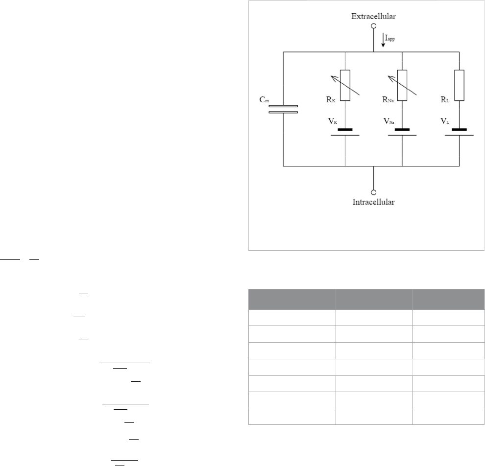
The conductance-based model describes the potential using the
currents passing through the membrane. Figure A1 shows the
electrical circuit that represents this phenomenon, which presents
a capacitor representing the membrane (C
m
), resistors and sources
to represent the ion channels (potassium V
K
, sodium V
Na
, and
others V
L
), and an applied current to indicate the stimulus from the
nervous system (I
app
).
Kirchhoff’s first law [47] was applied to the circuit shown in
Figure A1 to determinate Eq. A1, which describes the action
potential in the membrane, where
g
Na
,
g
K
, and
g
L
are the
conductance of the channels of sodium, potassium, and other
ions, V
Na
, V
K
, and V
L
are the potential differences of these
channels, and C
m
is the membrane conductance. Eqs A2–A4
represent the auxiliary variables n, m, and h, as described in [41].
These equations use alpha (α) and beta (β) functions, as also
described in [41], which are given in Eqs A5–A10. All constants
used for the membrane action potential model are given in Table A1.
dV
m
[]
dt
1
C
m
I
app
−
g
k
n
4
V
m
− V
k
()
−
g
Na
m
3
hV
m
− V
Na
()
−
g
l
V
m
− V
l
()
,
(A1)
dn
dt
α
n
1 − n
()
− β
n
n, (A2)
dm
dt
α
m
1 − m
()
− β
m
m, (A3)
dh
dt
α
h
1 − h
()
− β
h
h, (A4)
α
n
0.01 10 − V
m
()
e
10−V
m
10
− 1
, (A5)
β
n
0.125e
−V
m
80
, (A6)
α
m
0.125− V
m
()
e
25−V
m
10
− 1
, (A7)
β
m
4e
−V
m
18
, (A8)
α
h
0.07e
−V
m
20
, (A9)
β
h
1
e
−V
m
10
+ 1
. (A10)
FIGURE A1
Electric circuit representing the cellular membrane, as described
in [41].
TABLE A1 Input parameters for the action potential model.
Parameter Value Citation
C
m
1 μF/cm
2
[42]
g
Na
120 mS/cm
2
[42]
g
K
36 mS/cm
2
[42]
g
L
0.3 mS/cm
2
[42]
V
Na
115 mV [42]
V
K
−12 mV [42]
V
L
10.6 mV [42]
Frontiers in Physics frontiersin.org10
Kappaun et al. 10.3389/fphy.2023.1323542
