Wim Vanderbauwhede
Jeremy Singer
Operating Systems
Foundations
with Linux on the Raspberry Pi
TEXTBOOK
Operating Systems
Foundations
with Linux on the Raspberry Pi

Wim Vanderbauwhede
Jeremy Singer
Operating Systems
Foundations
with Linux on the Raspberry Pi
TEXTBOOK

Arm Educaon Media is an imprint of Arm Limited, 110 Fulbourn Road, Cambridge, CBI 9NJ, UK
Copyright © 2019 Arm Limited (or its aliates). All rights reserved.
No part of this publicaon may be reproduced or transmied in any form or by any means, electronic
or mechanical, including photocopying, recording or any other informaon storage and retrieval
system, without permission in wring from the publisher, except under the following condions:
Permissions
You may download this book in PDF format for personal, non-commercial use only.
You may
reprint or republish portions of the text for non-commercial, educational or research
purposes but only if there is an attribution to Arm Education.
This book and the individual contributions contained in it are protected under copyright by the
Publisher (other than as may be noted herein). Nothing in this license grants you any right to modify
the whole, or portions of, this book.
Notices
Knowledge and best practice in this field are constantly changing. As new research and experience
broaden our understanding, changes in research methods and professional practices may become
necessary.
Readers must always rely on their own experience and knowledge in evaluating and using any
information, methods, project work, or experiments described herein. In using such information or
methods, they should be mindful of their safety and the safety of others, including parties for whom
they have a professional responsibility.
To the fullest extent permitted by law, the publisher and the authors, contributors, and editors shall
not have any responsibility or liability for any losses, liabilities, claims, damages, costs or expenses
resulting from or suffered in connection with the use of the information and materials set out in this
textbook.
Such information and materials are protected by intellectual property rights around the world and are
copyright © Arm Limited (or its affiliates). All rights are reserved. Any source code, models or other
materials set out in this textbook should only be used for non-commercial, educational purposes (and/or
subject to the terms of any license that is specified or otherwise provided by Arm). In no event shall
purchasing this textbook be construed as granting a license to use any other Arm technology or know-how.
ISBN: 978-1-911531-21-0
Version: 1.0.0 – PDF
For information on all Arm Education Media publications, visit our website at www.armedumedia.com
To report errors or send feedback please email [email protected]

Foreword
xviii
Disclaimer
xix
Preface
xx
About the Authors
xxiv
Acknowledgments
xxv
1. A Memory-centric system model
1.1 Overview
2
1.2 Modeling the system
2
1.2.1 The simplest possible model
2
1.2.2 What is this ‘‘system state’’?
3
1.2.3 Rening non-processor acons
4
1.2.4 Interrupt requests
4
1.2.5 An important peripheral: the mer
5
1.3 Bare-bones processor model
5
1.3.1 What does the processor do?
5
1.3.2 Processor internal state: registers
6
1.3.3 Processor instrucons
7
1.3.4 Assembly language
8
1.3.5 Arithmec logic unit
8
1.3.6 Instrucon cycle
8
1.3.7 Bare bones processor model
10
1.4 Advanced processor model
11
1.4.1 Stack support
11
1.4.2 Subroune calls
12
1.4.3 Interrupt handling
13
1.4.4 Direct memory access
13
1.4.5 Complete cycle-based processor model
14
1.4.6 Caching
15
1.4.7 Running a program on the processor
18
1.4.8 High-level instrucons
19
1.5 Basic operang system concepts
20
1.5.1 Tasks and concurrency
20
1.5.2 The register le
21
1.5.3 Time slicing and scheduling
21
1.5.4 Privileges
23
Contents
vi

1.5.5 Memory management
23
1.5.6 Translaon look-aside buer (TLB)
24
1.6 Exercises and quesons
25
1.6.1 Task scheduling
25
1.6.2 TLB model
25
1.6.3 Modeling the system
25
1.6.4 Bare-bones processor model
25
1.6.5 Advanced processor model
25
1.6.6 Basic operang system concepts
25
2. A Praccal view of the Linux System
2.1 Overview
30
2.2 Basic concepts
30
2.2.1 Operang system hierarchy
31
2.2.2 Processes
31
2.2.3 User space and kernel space
32
2.2.4 Device tree and ATAGs
32
2.2.5 Files and persistent storage
32
Paron
32
File system
33
2.2.6 ‘Everything is a le’
33
2.2.7 Users
34
2.2.8 Credenals
34
2.2.9 Privileges and user administraon
35
2.3 Boong Linux on the Arm (Raspberry Pi 3)
36
2.3.1 Boot process stage 1: Find the bootloader
36
2.3.2 Boot process stage 2: Enable the SDRAM
36
2.3.3 Boot process stage 3: Load the Linux kernel into memory
37
2.3.4 Boot process stage 4: Start the Linux kernel
37
2.3.4 Boot process stage 5: Run the processor-independent kernel code
37
2.3.5 Inializaon
37
2.3.6 Login
38
2.4 Kernel administraon and programming
38
2.4.1 Loadable kernel modules and device drivers
38
2.4.2 Anatomy of a Linux kernel module
39
2.4.3 Building a custom kernel module
41
2.4.4 Building a custom kernel
42
Contents
vii

2.5 Kernel administraon and programming
42
2.5.1 Process management
42
2.5.2 Process scheduling
43
2.5.3 Memory management
43
2.5.4 Concurrency and parallelism
43
2.5.5 Input/output
43
2.5.6 Persistent storage
43
2.5.7 Networking
44
2.6 Summary
44
2.7 Exercises and quesons
44
2.7.1 Installing Raspbian on the Raspberry Pi 3
44
2.7.2 Seng up SSH under Raspbian
44
2.7.3 Wring a kernel module
44
2.7.4 Boong Linux on the Raspberry Pi
45
2.7.5 Inializaon
45
2.7.6 Login
45
2.7.7 Administraon
45
3. Hardware architecture
3.1 Overview
49
3.2 Arm hardware architecture
49
3.3 Arm Cortex M0+
50
3.3.1 Interrupt control
51
3.3.2 Instrucon set
51
3.3.3 System mer
52
3.3.4 Processor mode and privileges
52
3.3.5 Memory protecon
52
3.4 Arm Cortex A53
53
3.4.1 Interrupt control
53
3.4.2 Instrucon set
54
Floang-point and SIMD support
55
3.4.3 System mer
56
3.4.4 Processor mode and privileges
56
3.4.5 Memory management unit
57
Translaon look-aside buer
58
Addional caches
59
viii
Contents

3.4.6 Memory system
59
L1 Cache
59
L2 Cache
60
Data cache coherency
61
3.5 Address map
61
3.6 Direct memory access
63
3.7 Summary
64
3.8 Exercises and quesons
64
3.8.1 Bare-bones programming
64
3.8.2 Arm hardware architecture
65
3.8.3 Arm Cortex M0+
65
3.8.4 Arm Cortex A53
65
3.8.5 Address map
65
3.8.6 Direct memory access
65
4. Process management
4.1 Overview
70
4.2 The process abstracon
70
4.2.1 Discovering processes
71
4.2.2 Launching a new process
71
4.2.3 Doing something dierent
73
4.2.4 Ending a process
73
4.3 Process metadata
74
4.3.1 The /proc le system
75
4.3.2 Linux kernel data structures
76
4.3.3 Process hierarchies
77
4.4 Process state transions
79
4.5 Context switch
81
4.6 Signal communicaons
83
4.6.1 Sending signals
83
4.6.2 Handling signals
84
4.7 Summary
85
4.8 Further reading
85
4.9 Exercises and quesons
85
4.9.1 Mulple choice quiz
85
4.9.2 Metadata mix
86
Contents
ix

4.9.3 Russian doll project
86
4.9.4 Process overload
86
4.9.5 Signal frequency
86
4.9.6 Illegal instrucons
86
5. Process scheduling
5.1 Overview
90
5.2 Scheduling overview: what, why, how?
90
5.2.1 Denion
90
5.2.2 Scheduling for responsiveness
90
5.2.3 Scheduling for performance
91
5.2.4 Scheduling policies
91
5.3 Recap: the process lifecycle
91
5.4 System calls
93
5.4.1 The Linux syscall(2) funcon
94
5.4.2 The implicaons of the system call mechanism
95
5.5 Scheduling principles
95
5.5.1 Preempve versus non-preempve scheduling
96
5.5.2 Scheduling policies
96
5.5.3 Task aributes
96
5.6 Scheduling criteria
96
5.7 Scheduling policies
97
5.7.1 First-come, rst-served (FCFS)
97
5.7.2 Round-robin (RR)
98
5.7.3 Priority-driven scheduling
98
5.7.4 Shortest job rst (SJF) and shortest remaining me rst (SRTF)
99
5.7.5 Shortest elapsed me rst (SETF)
100
5.7.6 Priority scheduling
100
5.7.7 Real-me scheduling
100
5.7.8 Earliest deadline rst (EDF)
101
5.8 Scheduling in the Linux kernel
101
5.8.1 User priories: niceness
102
5.8.2 Scheduling informaon in the task control block (TCB)
102
5.8.3 Process priories in the Linux kernel
104
Priority info in task_struct
105
Priority and load weight
106
x
Contents

5.8.4 Normal scheduling policies: the completely fair scheduler (CFS)
107
5.8.5 So real-me scheduling policies
110
5.8.6 Hard real-me scheduling policy
112
Time budget allocaon
113
5.8.7 Kernel preempon models
115
5.8.8 The red-black tree in the Linux kernel
116
Creang a new rbtree
116
Searching for a value in a rbtree
117
Inserng data into a rbtree
117
Removing or replacing exisng data in a rbtree
118
Iterang through the elements stored in a rbtree (in sort order)
118
Cached rbtrees
119
5.8.9 Linux scheduling commands and API
119
Normal processes
119
Real-me processes
120
5.9 Summary
120
5.10 Exercises and quesons
120
5.10.1 Wring a scheduler
120
5.10.2 Scheduling
120
5.10.3 System calls
121
5.10.4 Scheduling policies
121
5.10.5 The Linux scheduler
121
6. Memory management
6.1 Overview
126
6.2 Physical memory
126
6.3 Virtual memory
127
6.3.1 Conceptual view of memory
127
6.3.2 Virtual addressing
128
6.3.3 Paging
129
6.4 Page tables
130
6.4.1 Page table structure
130
6.4.2 Linux page tables on Arm
132
6.4.3 Page metadata
134
6.4.4 Faster translaon
136
6.4.5 Architectural details
137
Contents
xi

6.5 Managing memory over-commitment
138
6.5.1 Swapping
138
6.5.2 Handling page faults
138
6.5.3 Working set size
141
6.5.4 In-memory caches
142
6.5.5 Page replacement policies
142
Random
143
Not recently used (NRU)
143
Clock
143
Least recently used
144
Tuning the system
144
6.5.6 Demand paging
145
6.5.7 Copy on Write (CoW)
146
6.5.8 Out of memory killer
147
6.6 Process view of memory
148
6.7 Advanced topics
149
6.8 Further reading
151
6.9 Exercises and quesons
151
6.9.1 How much memory?
151
6.9.2 Hypothecal address space
152
6.9.3 Custom memory protecon
152
6.9.4 Inverted page tables
152
6.9.5 How much memory?
153
6.9.6 Tiny virtual address space
153
6.9.7 Denions quiz
153
7. Concurrency and parallelism
7.1 Overview
158
7.2 Concurrency and parallelism: denions
158
7.2.1 What is concurrency?
158
7.2.2 What is parallelism?
158
7.2.3 Programming model view
158
7.3 Concurrency
159
7.3.1 What are the issues with concurrency?
159
Shared resources
159
Exchange of informaon
160
xii
Contents
7.3.2 Concurrency terminology
161
Crical secon
161
Synchronizaon
161
Deadlock
161
7.3.3 Synchronizaon primives
163
7.3.4 Arm hardware support for synchronizaon primives
163
Exclusive operaons and monitors
163
Shareability domains
164
7.3.5 Linux kernel synchronizaon primives
165
Atomic primives
165
Memory operaon ordering
169
Memory barriers
170
Spin locks
173
Futexes
174
Kernel mutexes
174
Semaphores
175
7.3.6 POSIX synchronizaon primives
177
Mutexes
178
Semaphores
178
Spin locks
179
Condion variables
179
7.4 Parallelism
181
7.4.1 What are the challenges with parallelism?
181
7.4.2 Arm hardware support for parallelism
182
7.4.3 Linux kernel support for parallelism
183
SMP boot process
183
Load balancing
183
Processor anity control
184
7.5 Data-parallel and task-parallel programming models
184
7.5.1 Data parallel programming
184
Full data parallelism: map
184
Reducon
185
Associavity
185
Binary tree-based parallel reducon
185
7.5.2 Task parallel programming
186
Contents
xiii

7.6 Praccal parallel programming frameworks
186
7.6.1 POSIX Threads (pthreads)
186
7.6.2 OpenMP
189
7.6.3 Message passing interface (MPI)
190
7.6.4 OpenCL
191
7.6.5 Intel threading building blocks (TBB)
194
7.6.6 MapReduce
195
7.7 Summary
195
7.8 Exercises and quesons
195
7.8.1 Concurrency: synchronizaon of tasks
196
7.8.1 Parallelism
196
8. Input/output
8.1 Overview
202
8.2 The device zoo
202
8.2.1 Inspect your devices
203
8.2.2 Device classes
203
8.2.3 Trivial device driver
204
8.3 Connecng devices
206
8.3.1 Bus architecture
206
8.4 Communicang with devices
207
8.4.1 Device abstracons
207
8.4.2 Blocking versus non-blocking IO
207
8.4.3 Managing IO interacons
208
Polling
209
Interrupts
209
Direct memory access
210
8.5 Interrupt handlers
210
8.5.1 Specic interrupt handling details
211
8.5.2 Install an interrupt handler
212
8.6 Ecient IO
213
8.7 Further reading
213
8.8 Exercises and quesons
213
8.8.1 How many interrupts?
213
8.8.2 Comparave complexity
214
8.8.3 Roll your own Interrupt Handler
214
8.8.4 Morse Code LED Device
214
xiv
Contents

9. Persistent storage
9.1 Overview
218
9.2 User perspecve on the le system
218
9.2.1 What is a le?
218
9.2.2 How are mulple les organized?
219
9.3 Operaons on les
221
9.4 Operaons on directories
222
9.5 Keeping track of open les
222
9.6 Concurrent access to les
223
9.7 File metadata
225
9.8 Block-structured storage
226
9.9 Construcng a logical le system
228
9.9.1 Virtual le system
228
9.10 Inodes
230
9.10.1 Mulple links, single inode
231
9.10.2 Directories
231
9.11 ext4
233
9.11.1 Layout on disk
233
9.11.2 Indexing data blocks
224
9.11.3 Mulple links, single inode
237
9.11.4 Checksumming
237
9.11.5 Encrypon
237
9.12 FAT
238
9.12.1 Advantages of FAT
239
9.12.2 Construct a mini le system using FAT
240
9.13 Latency reducon techniques
242
9.14 Fixing up broken le systems
243
9.15 Advanced topics
243
9.16 Further reading
245
9.17 Exercises and quesons
245
9.17.1 Hybrid conguous and linked le system
245
9.17.2 Extra FAT le pointers
245
9.17.3 Expected le size
245
9.17.4 Ext4 extents
245
9.17.5 Access mes
245
9.17.6 Database decisions
246
Contents
xv

10. Networking
10.1 Overview
250
10.2 What is networking
250
10.3 Why is networking part of the kernel?
250
10.4 The OSI layer model
251
10.5 The Linux networking stack
252
10.5.1 Device drivers
253
10.5.2 Device-agnosc interface
253
10.5.3 Network protocols
253
10.5.4 Protocol-agnosc interface
253
10.5.5 System call interface
254
10.5.6 Socket buers
254
10.6 The POSIX standard socket interface library
255
10.6.1 Stream socket (TCP) communicaons ow
255
10.6.2 Common internet data types
256
Socket address data type: struct sockaddr
256
Internet socket address data type: struct sockaddr_in
257
10.6.3 Common POSIX socket API funcons
258
Create a socket descriptor: socket()
258
Bind a server socket address to a socket descriptor: bind()
258
Enable server socket connecon requests: listen()
259
Accept a server socket connecon request: accept()
259
Client connecon request: ‘connect()’
260
Write data to a stream socket: send()
261
Read data from a stream socket: recv()
261
Seng server socket opons: setsockopt()
262
10.6.4 Common ulity funcons
263
Internet address manipulaon funcons
263
Internet network/host byte order manipulaon funcons
263
Host table access funcons
264
10.6.5 Building applicaons with TCP
264
Request/response communicaon using TCP
264
TCP server
265
TCP client
266
10.6.6 Building applicaons with UDP
268
UDP server
269
xvi
Contents

UDP client
270
UDP client using connect()
271
10.6.7 Handling mulple clients
271
The select() system call
271
Mulple server processes: fork() and exec()
275
Multhreaded servers using pthreads
276
10.7 Summary
278
10.8 Exercises and quesons
278
10.8.1 Simple social networking
278
10.8.2 The Linux networking stack
278
10.8.3 The POSIX socket API
278
11. Advanced topics
11.1 Overview
282
11.2 Scaling down
282
11.3 Scaling up
283
11.4 Virtualizaon and containerizaon
285
11.5 Security
287
11.5.1 Rowhammer, Rampage, Throwhammer, and Nethammer
287
11.5.2 Spectre, Meltdown, Foreshadow
288
11.6 Vericaon and cercaon
289
11.7 Recongurability
291
11.8 Linux development roadmap
292
11.9 Further reading
293
11.10 Exercises and quesons
293
11.10.1 Make a minimal kernel
293
11.10.2 Verify important properes
293
11.10.3 Commercial comparison
293
11.10.4 For or against cercaon
293
11.10.5 Devolved decisions
293
11.10.6 Underclock, overclock
293
Glossary of terms
296
Index
304
Contents
xvii
Foreword
In 1983, when I started modeling a RISC processor using a simulator wrien in BBC Basic on a BBC
Microcomputer, I could hardly have conceived that there would be billions of Arm (then short for
‘Acorn RISC Machine’) processors all over the world within a few decades.
I expect Linus Torvalds has similar feelings, when he thinks back to the early days, craing a prototype
operang system for his i386 PC. Now Linux runs on a vast array of devices, from smartwatches to
supercomputers. I am delighted that an increasing proporon of these devices are built around Arm
processor cores.
In a more recent tale of runaway success, the Raspberry Pi single-board computer has far exceeded
its designers’ inial expectaons. The Raspberry Pi Foundaon thought they might sell one thousand
units, ‘maybe 10 thousand in our wildest dreams.’ With sales gures now around 20 million, the
Raspberry Pi is rmly established as Britain’s best-selling computer.
This textbook aims to bring these three technologies together—Arm, Linux, and Raspberry Pi. The
authors’ ambious goal is to ‘make Operang Systems fun again.’ As a professor in one of the UK’s
largest university Computer Science departments, I am well aware that modern students demand
engaging learning materials. Dusty 900-page textbooks with occasional black and white illustraons
are not well received. Today’s learners require interacve content, gaining understanding through
praccal experience and intuive analogies. My observaon applies to students in tradional higher
educaon, as well as those pursuing blended and fully online educaon. I am condent this innovave
textbook will meet the needs of the next generaon of Computer Science students.
While the modern systems soware stack has become large and complex, the fundamental principles
are unchanging. Operang Systems must trade-o abstracon for eciency. In this respect, Linux
on Arm is parcularly instrucve. The authors do an excellent job of presenng Operang Systems
concepts, with direct links to concrete examples of these concepts in Linux on the Raspberry Pi.
Please don’t just read this textbook – buy a Pi and try out the praccal exercises as you go.
Was it Plutarch who said, ‘The mind is not a vessel to be lled but a re to be kindled’? We could
translate this into the Operang Systems domain as follows: ‘Learning isn’t just reading source code;
it’s bootstrapping machines.’ I hope that you enjoy all these acvies, as you explore Operang
Systems with Linux on Arm using your Raspberry Pi.
Steve Furber CBE FRS FREng
ICL Professor of Computer Engineering
The University of Manchester, UK
February 2019
xviii
xix
Disclaimer
The design examples and related soware les included in this book are created for educaonal
purposes and are not validated to the same quality level as Arm IP products. Arm Educaon Media
and the author do not make any warranes of these designs.
Note
When we developed the material for this textbook, we worked with Raspberry Pi 3B boards.
However, all our praccal exercises should work on other generaons and variants of Raspberry Pi
devices, including the more recent Raspberry Pi 4.
Preface
Introducon
Modern computer devices are fabulously complicated both in terms of the processor hardware and
the soware they run.
At the heart of any modern computer device sits the operang system. And if the device is a
smartphone, IoT node, datacentre server or supercomputer, then the operang system is very likely to
be Linux: about half of consumer devices run Linux; the vast majority of smartphones worldwide (86%)
run Android, which is built on the Linux kernel. Of the top one million web servers, 98% run Linux.
Finally, the top 500 fastest supercomputers in the world all run Linux.
On the hardware side, Arm has a 95% market share in smartphone and tablet processors as well as
being used in the majority of Internet of Things (IoT) devices such as webcams, wireless routers, etc.
and embedded devices in general.
Since its creaon by Linus Torvalds in 1991, the eorts of thousands of people, most of them
volunteers, have turned Linux into a state-of-the-art, exible and powerful operang system, suitable
for any system from ny IoT devices to the most powerful supercomputers.
Meanwhile, in roughly the same period, the Arm processor range has expanded to cover an equally
wide gamut of systems and devices, including the remarkably successful Raspberry Pi.
So if you want to learn about Operang Systems but keep a praccal, real-world focus, then this book
is an ideal starng point. This book will help you answer quesons such as:
What is a le, and why is the le concept so important in Linux?
What is scheduling and how can knowledge of Linux scheduling help you create a high-throughput
video processor or a mission-crical real-me system?
What are POSIX threads, and how can the Linux kernel assist you in making your multhreaded
applicaons faster and more responsive?
How does the Linux kernel support networking, and how do you create network clients and servers?
How does the Arm hardware assist the Linux kernel in managing memory and how does
understanding memory management make you a beer programmer?
The aim of this book is to provide a praccal introducon to the foundaons of modern operang
systems, with a parcular focus on GNU/Linux and the Arm plaorm. Our unique perspecve is
that we explain operang systems theory and concepts but ground them in praccal use through
illustrave examples of their implementaon in GNU/Linux, as well as making the connecon with
the Arm hardware supporng the OS funconality.
xx

Is this book suitable for you?
This book does not require prior knowledge of operang systems, but some familiarity with command-
line operaons in a GNU/Linux system is expected. We discuss technical details of operang systems,
and we use source code to illustrate many concepts. Therefore, you need to know C and Python, and
you need to be familiar with basic data structures such as arrays, queues, stacks and trees.
This textbook is ideal for a one-semester course introducing the concepts and principles underlying
modern operang systems. It complements the Arm online courses in Real-Time Operang Systems
Design and Programming, and Embedded Linux.
Online addional material
The companion web site of the book (www.dcs.gla.ac.uk/operang-system-foundaons) contains:
Source code for all original code snippets listed in the book;
Answers to quesons and exercises;
Lab materials;
Addional content;
Addional teaching materials;
Further reading.
Target plaorm
This textbook focuses on the Raspberry Pi 3, an Arm Cortex-A53 plaorm running Linux. We use the
Raspbian GNU/Linux distribuon. However, the book does not specically depend on this plaorm
and distribuon, except for the exercises.
If you don’t own a Raspberry Pi 3, you can use the QEMU emulator which supports the Raspberry Pi 3.
Soware development environment
The code examples in this book are either in C or Python 3. We assume that the reader has access
to a Linux system with an installaon of Python, a C compiler, the make build tool and the git version
control tool.
Structure
The structure of this textbook is based on our many years of teaching operang systems courses at
undergraduate and masters level, taking into account the feedback provided by the reviewers of the
text. The content of the text is closely aligned to the Compung Curricula 2001 Compung Science
report recommendaons for teaching Operang Systems, published by the Joint Task Force of the
IEEE Compung Society and the Associaon for Compung Machinery (ACM).
xxi
Preface

The book is organized into eleven chapters.
Chapters 1 and 2 provide alternate introductory views to operang systems.
Chapter 1 A memory-centric system model presents a top-down view. In this chapter, we introduce a
number of abstract models for processor-based systems. We use Python code to describe the models
and only use simple data structures and funcons. The purpose is to help the student understand that
in a processor-based system, all acons fundamentally reduce to operaons on addresses. The models
are gradually being rened as the chapter advances, and by the end, the model integrates the basic
operang system funconality into a runnable Python-based processor model.
Chapter 2 A praccal view of the Linux system approaches the Linux system from a praccal
perspecve: what actually happens when we boot and run the system, how does it work and what is
required to make it work. We rst introduce the essenal concepts and techniques that the student
needs to know in order to understand the overall system, and then we discuss the system itself.
The aim of this part is to help the student answer quesons such as “what happens when the system
boots?” or “how does Linux support graphics?”. This is not a how-to guide, but rather, provides the
student with the background knowledge behind how-to guides.
In Chapter 3 Hardware architecture, we discuss the hardware on which the operang system runs,
the hardware support for operang systems (dedicated registers, MMU, DMA, interrupt architecture,
relevant details about the bus/NoC architecture, ...), the memory subsystem (caches, TLB), high-level
language support, boot subsystem and boot sequence. The purpose is to provide the student with a
useable mental model for the hardware system and to explain the need for an operang system and
how the hardware supports the OS. In parcular, we study the Linux view on the hardware system.
The next seven chapters form the core of the book, each of these introduces a core Operang System
concept.
In Chapter 4, Process management, we introduce the process abstracon. We outline the state
that needs to be encapsulated. We walk through the typical lifecycle of a process from forking to
terminaon. We review the typical operaons that will be performed on a process.
Chapter 5 Process scheduling discusses how the OS schedules processes on a processor. This includes
the raonale for scheduling, the concept of context switching, and an overview of scheduling policies
(FCFS, priority, ...) and scheduler architectures (FIFO, mullevel feedback queues, priories, ...). The
Linux scheduler is studied in detail.
While memory itself is remarkably straighorward, OS architects have built lots of abstracon layers
on top. Principally, these abstracons serve to improve performance and/or programmability. In
Chapter 6 Memory management, we review caches (in hardware and soware) to improve access
speed. We go into detail about virtual memory to improve the management of physical memory
resource. We will provide highly graphical descripons of address translaon, paging, page tables,
page faults, swapping, etc. We explore standard schemes for page replacement, copy-on-write, etc.
We will examine concrete examples in Arm architecture and Linux OS.
xxii
Preface

In Chapter 7, Concurrency and parallelism, we discuss how the OS supports concurrency and how the
OS can assist in exploing hardware parallelism. We dene concurrency and parallelism and discuss
how they relate to threads and processes. We discuss the key issue of resource sharing, covering
locking, semaphores, deadlock and livelock. We look at OS support for concurrent and parallel
programming via POSIX threads and present an overview of praccal parallel programming techniques
such as OpenMP, MPI and OpenCL.
Chapter 8 Input/output presents the OS abstracon of an IO device. We review device interfacing,
covering topics like Polling, Interrupts and DMA. We will invesgate a range of device types, to
highlight their diverse features and behavior. We will cover hardware registers, memory mapping
and coprocessors. Further, we will examine the ways in which devices are exposed to programmers.
We will review the structure of a typical device driver.
Chapter 9 Persistent storage focuses on data storage. We outline the range of use cases for le
systems. We explain how the raw hardware (block- and sector-based 2d storage, etc.) is abstracted at
the OS level. We talk about mapping high-level concepts like les, directories, permissions, etc., down
to physical enes. We review allocaon, space management, and recovery from failure. We present
a case study of a Linux le system. We also discuss Windows-style FAT, since this is how USB bulk
storage operates.
Chapter 10 Networking introduces networking from an OS perspecve: why is networking treated
dierently from other types of IO, what are the OS requirements to support the OSI stack. We
introduce socket programming with a focus of the role the OS plays (e.g. zero-copy buers, le
abstracon, supporng mulple clients, ...).
Finally, Chapter 11 Advanced topics discusses a number of concepts that go beyond the material of
the previous chapters: The rst part of this chapter deals with customisaon of Linux for Embedded
Systems, Linux on systems without MMU, and datacentre level operang systems. The second
part discusses the security of Linux-based systems, focusing on validaon and vericaon of OS
components and the analysis of recent security exploits.
We hope that you enjoy both reading our book and doing the exercises – especially if you are trying
them on the Raspberry Pi. Please do let us know what you think about our work and how we could
improve it by sending your comments to Arm Educaon Media [email protected]
Jeremy Singer and Wim Vanderbauwhede, 2019
xxiii
Preface
About the Authors
Wim Vanderbauwhede
School of Compung Science, University of Glasgow, UK
Prof. Wim Vanderbauwhede is Professor in Compung Science at the School of Compung Science
of the University of Glasgow. He has been teaching and researching operang systems for over
a decade. His research focuses on high-level programming, compilaon, and architectures for
heterogeneous manycore systems and FPGAs, with a special interest in power-ecient compung
and scienc High-Performance Compung (HPC). He is the author of the book ‘High-Performance
Compung Using FPGAs’. He received his Ph.D. in Electrotechnical Engineering with Specialisaon
in Physics from the University of Gent, Belgium in 1996. Before moving into academic research,
Prof. Vanderbauwhede worked as an ASIC Design Engineer and Senior Technology R&D Engineer for
Alcatel Microelectronics.
Jeremy Singer
School of Compung Science, University of Glasgow, UK
Dr. Jeremy Singer is a Senior Lecturer in Systems at the School of Compung Science of the University
of Glasgow. His main research theme involves programming language runmes, with parcular
interests in garbage collecon and manycore parallelism. He leads the Federated Raspberry Pi
Micro-Infrastructure Testbed (FRµIT) team, invesgang next-generaon edge compute plaorms.
He received his Ph.D. from the University of Cambridge Computer Laboratory in 2006. Singer and
Vanderbauwhede also collaborated in the design of the FutureLearn ‘Funconal Programming in
Haskell’ massive open online course.
xxiv
Acknowledgements
The authors would like to thank the following people for their help:
Khaled Benkrid, who made this book possible.
Ashkan Tousimojarad, who originally suggested the project.
Melissa Good, Jialin Dou and Michael Shu who kept us on track and assisted us with the process.
The reviewers at Arm who provided valuable feedback on our dras.
Tony Garnock-Jones, Dejice Jacob, Richard Morer, Colin Perkins, and other colleagues who
commented on early versions of the text.
Steve Furber, for his kind endorsement of the book.
Lovisa Sundin, for her help with illustraons.
Jim Garside, Krisan Hentschel, Simon McIntosh-Smith, Magnus Morton and Michèle Weiland for
kindly allowing us to use their photographs.
The countless volunteers who made the Linux kernel what it is today.
xxv

Chapter 1
A Memory-centric
system model

Operang Systems Foundaons with Linux on the Raspberry Pi
2
1.1 Overview
In this chapter, we will introduce a number of abstract memory-centric models for processor-based
systems. We will use Python code to describe the models and only use simple data structures and
funcons. The models are abstract in the sense that we do not build the processor system starng from
its physical building blocks (transistors, logic gates, etc.), but rather, we model it in a funconal way.
The purpose is to help you understand that in a processor-based system, all acons fundamentally
reduce to operaons on addresses. This is a very important point: every observable acon in a processor-
based system is the result of wring to or reading from an address locaon.
In parcular, this includes all peripherals of the system, such as the network card, keyboard, and display.
What you will learn
Aer you have studied the material in this chapter, you will be able to:
1. Discuss the importance of state and the address space in a processor-based system.
2. Create a processor-based system model in a high-level language.
3. Implement basic operang system concepts such as me slicing in machine code.
4. Explain how hardware and soware features of a processor-based system are designed to handle
I/O, concurrency, and performance.
1.2 Modeling the system
A microprocessor is driven by a clock.
Our model will describe the acons at every ck of the clock using funcons.
We will model the system through its state, represented as a simple data structure.
By “state,” we mean informaon that is persistent, i.e., some form of memory. This is not limited to
actual computer memory. For example, if our system controls a robot arm, then the posion of the
arm is part of the state of the system.
1.2.1 The simplest possible model
We start our system model by stang that the acon of the processor modies the system state:
systemState = processorAction(systemState)
Python
In pracce, the system also interacts with the outside world through peripherals such as the keyboard,
network interface, etc., generally called “I/O devices”, storage devices such as disks, etc. Let's just call
these types of acons to modify the state ‘non-processor acons’. Adding this to our model, we get:

3
Lisng 1.2.1: System state with non-processor acons Python
1 systemState = nonProcessorAction(systemState)
2 systemState systemState = processorAction(systemState)
In a real system, these acons happen at the same me (we call concurrent acons), so one of the
quesons (that we will address in detail in Chapters 7, ‘Concurrency and parallelism’) is how to make
sure that the system state does not become undetermined as a result of concurrent acons. But rst,
let’s look in a bit more detail at the system state.
1.2.2 What is this ‘system state’?
We say that the processor ‘‘modies the system state’’, so let’s take a closer look at this system
state. From the point of view of the processor, the system state is simply a xed-size array of unsigned
integers. Nothing more than that. In C syntax, we can express this as shown in Lisng 1.2.2:
Lisng 1.2.2: System state as C array C
1 int systemState[STATE_SZ]
Which means that manipulaon of the system state, and by consequence, anything that happens in
a processor-based system boils down to modifying this array.
So, what does this array actually represent? It represents all of the memory in the system, not just the
actual system memory (DRAM, Dynamic Random Access Memory) but including the I/O devices and
other peripherals such as disks. In system terms, this is known as the ‘physical address space’, and we
will discuss this in detail in Chapter 6, ‘‘Memory management.’’
1
In other words, the system state is composed of the states of all the system components, for example
for a system with a keyboard kbd, network interface card nic, solid state disk ssd, graphics processing
unit gpu, and random access memory ram:
systemState = ramState + kbdState + nicState + ssdState + gpuState
Python
Where ramState, kbdState, nicState, etc. are all xed-size arrays of integers.
However, it could of course equally be:
systemState = ssdState + kbdState + nicState + ramState + gpuState
Python
The above are two examples of address space layouts. The descripon of the purpose, size, and
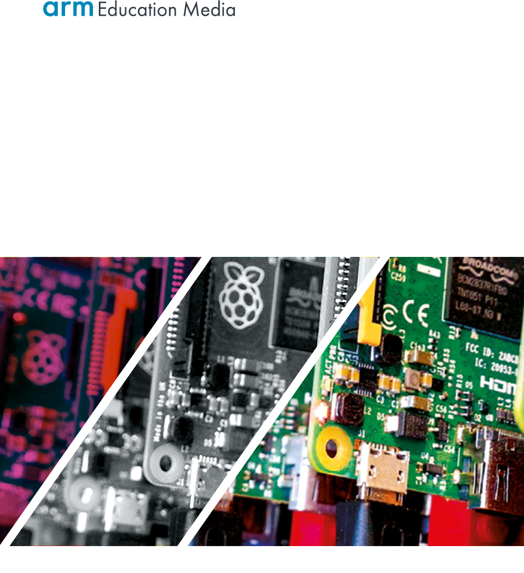
posion of the address regions for memory and peripherals is called the address map. As an illustraon,
the Arm address map for A-class systems [1] is shown in Figure 1.1.
1
As our model focuses on Arm-based systems, we do not discuss port-mapped I/O.
Chapter 1 | A Memory-centric system model
Operang Systems Foundaons with Linux on the Raspberry Pi
4
Figure 1.1: Arm 40-bit address map.
Figure 1.1. If the address size is 32 bits, we can address 2
32
= 4GB of memory. We see from the gure
that dierent regions are reserved for dierent purposes, e.g., the second GB is memory mapped I/O,
and the upper 2 GB are random access memory (DRAM).
1.2.3 Rening non-processor acons
Using the more detailed state from above, we can split the non-processor acons into per-peripheral
acons, so that our model becomes:
Lisng 1.2.3: Model with per-peripheral acons Python
1 kbdState=kbdAction(kbdState)
2 nicState=nicAction(nicState)
3 ssdState=ssdAction(ssdState)
4 gpuState=gpuAction(gpuState)
5 systemState = ramState+kbdState+nicState+diskState+gpuState
6 systemState = processorAction(systemState)
Each of these acons only aects the state of the peripheral; the rest of the system state remains
unaected.
1.2.4 Interrupt requests
Let’s return now to the potenal problem of state modied by concurrent acons. The way we just
separated the state oers a possible soluon. Now we can create a kind of nocaon mechanism
which lets the processor know that an outside acon has modied the state
2
.
This is exactly what happens in real systems, and the mechanisms used are called interrupts. We will
discuss this in detail in Chapter 8, ‘Input/output’, but it is useful to add an interrupt mechanism to our
abstract model.
A peripheral can send an interrupt request (IRQ) to the processor. We will model the interrupt request as a
boolean ag which is returned by every peripheral acon together with its state (as a tuple). The processor
0 GB
1 GB
2 GB
4 GB
8 GB
16 GB
32 GB
64 GB
128 GB
256 GB
512 GB
1024 GB
32-bit
36-bit
40-bit
Mapped I/O
DRAM
Reserved
Mapped I/O
DRAM
Reserved
Mapped I/O
2 GB of DRAM
ROM & RAM & I/O
32-bit 36-bit 40-bit
0
32-bit
36-bit
40-bit
32 GB hole or DRAM
2 GB hole or DRAM
Log2 scale
2
We could also let the processor check if the state of a peripheral was changed before acng on it. This approach is called polling and will be discussed in Chapter 8, ‘Input/output’.

5
acon receives an array of these interrupt requests and uses the array index to idenfy the peripheral that
raised the interrupt (‘raising an interrupt’ in our model means seng the boolean ag to True).
In pracce, the mechanism is more complicated because many peripherals can raise mulple dierent
interrupt requests depending on the condion. Typically, a dedicated peripheral called interrupt
controller is used to manage the interrupts from the various devices.
Note that the interrupt mechanism is purely a nocaon mechanism: it does not stop the processor
from modifying the peripheral state, all it does is nofy the processor that the peripheral unilaterally
changed its state. So in principle, the peripheral could sll be modifying its state at the very same me
that the processor is modifying it. In what follows, we simply assume that this cannot happen, i.e., if a
peripheral is modifying its state, then the processor can’t change it and vice versa. A possible model for
this is that the peripheral state change and the interrupt request are happening at the same me and
that the processor always needs to process the request before making a state change.
Lisng 1.2.4: Model with interrupt requests Python
1 (kbdState,kbdIrq)=kbdAction(kbdState)
2 ...
3
4 irqs=[kbdIrq,...]
5
6 systemState = ramState+kbdState+nicState+diskState+gpuState
7 (systemState,irqs) = processorAction(systemState,irqs)
We will see in the next secon how the processor handles interrupts.
1.2.5 An important peripheral: the mer
A mer is a peripheral that counts me in terms of the system clock. It can be programmed to ‘re’
periodically at given intervals, or aer a one-o interval. When a mer ‘res’ it raises an interrupt
request. The mer is parcularly important because it is the principal mechanism used by the
operang system to track the progress of me and allows it to schedule tasks.
(timerState, timerIrq)=timerAction(timerState)
Python
1.3 Bare-bones processor model
To gain more insight into the way the processor modies the system state, we will build a simple processor
model which models how the processor changes the system state at every clock cycle. The purpose of
this model is to make the introducon of the more abstract model in Secon 1.4 easier to understand.
1.3.1 What does the processor do?
The processor is a machine to modify the system state. You need to know that …
A key feature of a processor is the ability to run arbitrary programs.
A program consists of a series of instrucons.
Chapter 1 | A Memory-centric system model
Operang Systems Foundaons with Linux on the Raspberry Pi
6
An instrucon determines how the processor interacts with the system through the address space: it can
read values at given addresses, compute new values and addresses, and write values to given addresses.
Note that the program is itself part of the system state. The program running on the processor can control
which part of the enre program code to access. This is what allows us to create an operang system.
1.3.2 Processor internal state: registers
Although in principle, a processor could directly manipulate the system state, this is not praccal
because DRAM memory access is quite slow. Therefore, in pracce, processors have a dedicated
internal state known as the register le, an array of words called registers which you can consider
as a small but very fast memory. The register le is separate from the rest of the system state (it is
a ‘separate address space’). This means we have to rene our model to separate the register le from
the rest of the system state, which we will call systemState. We do this using a tuple
3
:
(systemState,irqs,registers) = processorAction(systemState,irqs,registers)
Python
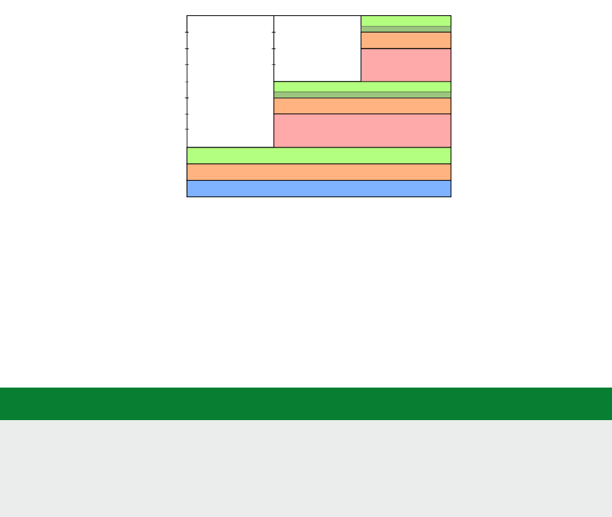
For convenience, registers oen have names (mnemonics). For example, Figure 1.2 shows the core
AArch32 register set of the Arm Cortex-A53 [2].
There are 16 ordinary registers (and ve special ones which we have omied). Registers R0-R12 are
the ‘General-purpose registers’. Then there are three registers with special names: the Stack Pointer
(SP), the Link Register (LR) and the Program Counter (PC).
Figure 1.2: Arm Cortex-A53 AArch32 register set.
3
Alternavely, we could make the registers part of the system state similar to the state of the peripherals. Our choice is purely for convenience because it makes it easier
to manipulate the registers in the Python code.
SP (R13)
LR (R14)
PC (R15)
R5
R6
R7
R0
R1
R3
R4
R2
R10
R11
R12
R8
R9
Low registers
High registers
General-purpose
registers
Stack Pointer
Link Register
Program Counter

7
1.3.3 Processor instrucons
A typical processor can perform a wide range of instrucons on memory addresses and/or register
values. We will use a simple list-based notaon for all instrucons. We will use the (uppercase) Arm
mnemonics for registers and instrucons; in Python, these are simply variables; their denions can
be found in the code repository in le abstract_system_constants.py.
We will assume that all instrucons take up to three registers as arguments, for example
add_instr = [ADD,R3,R1,R2]
Python
which means that the result of ADD operang on registers R1 and R2 is stored in register R3.
Apart from computaonal (arithmec and logic) instrucons we also introduce the instrucons LDR, e.g.
load_instr = [LDR,R1,R2]
Python
and STR, e.g.
store_instr=[STR,R1,R2]
Python
which respecvely load the content of a memory address stored in R2 into register R1 and store the
content of register R1 at the address locaon given in R2.
We also have MOV, which copies data between two registers, e.g.
set_instr = [MOV,R1,R2]
Python
will set the content of R1 to the content of R2.
We have a special non-Arm instrucon called SET, which takes a register and a value as arguments, e.g.
set_instr = [SET,R1,42]
Python
will set the content of R1 to 42.
We also need some instrucons to control the ow of the program, such as branches (B)
goto_instr = [B,R1]
Python
where R1 contains the address of the target instrucon in the program, and condional branches
(CBZ, ‘Compare and Branch if Zero’)
if_instr = [CBZ,R1,R2]
Python
where register R1 contains the condion variable (0 or 1) and the program branches to the address in R2 if
R1=0 and connues on the next line otherwise. We also have CBNZ, ‘Compare and Branch if Non-Zero’.
Chapter 1 | A Memory-centric system model

Operang Systems Foundaons with Linux on the Raspberry Pi
8
Finally, we have two instrucons which take no arguments: NOP does nothing, and WFI stops the
processor unl an interrupt occurs.
1.3.4 Assembly language
To write instrucons for actual processors, a similar, but more expressive, notaon called assembly
language is used. For example, consider the following program that reads two values from memory,
stores them in registers, adds them, and writes the result back:
Lisng 1.3.1: Example program Python
1 [
2 [LDR,R1,R4],
3 [LDR,R2,R5],
4 [ADD,R3,R1,R2],
5 [STR,R3,R6]
6 ]
In the assembly language for the Arm processor [3], this code would look as follows:
Lisng 1.3.2: Example Arm assembly program Python
1 ldr r1, r4
2 ldr r2, r5
3 add r3, r1, r2
4 str r3, r6
Assembly languages have many other features, such as a rich set of addressing mechanisms, labeling
opons, etc. However, for our current purpose, our simple funcon-based notaon is sucient. For
more details, see, e.g., [4].
1.3.5 Arithmec logic unit
The part of a processor that performs computaons is known as the arithmec logic unit (ALU).
We can create a simple ALU in Python as follows:
Lisng 1.3.3: ALU model Python
1 from operator import *
2
3 alu = [
4 add,
5 sub,
6 mul,
7 ...
8 ]
This is simply an array of funcons; more instrucons can be added trivially.
1.3.6 Instrucon cycle
A processor operates what is known as the instrucon cycle or fetch-decode-execute cycle. We can
dene each of these operaons as follows. First, we dene fetchInstrucon. This funcon fetches an

9
instrucon from memory. To determine which instrucon to fetch, it uses a dedicated register known
as the program counter, which has address PC in our register le. Then we also need to know where in
our memory space, we can nd the program code. We use CODE to denote the starng address of the
program in the system state. Aer reading the instrucon, we increment the program counter, so it
points to the next instrucon in the program.
Lisng 1.3.4: Instrucon fetch model Python
1 def fetchInstruction(registers,systemState):
2 # get the program counter
3 pctr = registers[PC]
4 # get the corresponding instruction
5 ir = systemState[CODE+pctr]
6 # increment the program counter
7 registers[PC]+=1
8 return ir
The instrucon is stored in the temporary instrucon register (ir in our code). The processor now has to
decode this instrucon, i.e., extract the register addresses and instrucon opcode from the instrucon
word. Remember that the state stores unsigned integers, so an instrucon is encoded as an unsigned
integer. The details of the implementaon can be found in the repository in le abstract_system_cpu_
decode.py. For this discussion, the important point is that the funcon returns a tuple opcode,args
where args is a tuple containing the decoded arguments (registers, addresses or constants). In the
code, if an element of a tuple is unused, we used _ as variable name to indicate this.
Lisng 1.3.5: Instrucon decode model Python
1 def decodeInstruction(ir):
2 ...
3 return (opcode,args)
Finally, the processor executes the decoded instrucon. In our model, we implement instrucon using
a funcon. The load instrucon (mnemonic LDR) is simply an array read operaon, store (mnemonic
STR) is simply an array write operaon. The B and CBZ branching instrucons only modify the program
counter. By using an array of funcons alu as discussed above, the ALU execuon is very simple too.
The complete code can be found in the repository in le abstract_- system_cpu_execute.py.
Lisng 1.3.6: Individual instrucon execute model Python
1 def doLDR(registers,systemState,args):
2 (r1,addr,_)=args
3 registers[r1] = systemState[addr]
4 return (registers,systemState)
5
6 def doSTR(registers,systemState,args)
7 (r1,addr,_)=args
8 systemState[addr]=registers[r1]
9 return (registers,systemState)
Chapter 1 | A Memory-centric system model

Operang Systems Foundaons with Linux on the Raspberry Pi
10
10
11 def doB(registers,args):
12 (_,addr,_)=args
13 registers[PC] = addr
14 return registers
15
16 def doCBZ(registers,args):
17 (r1,addr1,addr2)=args
18 if registers[r1]:
19 registers[PC] = addr1
20 else:
21 registers[PC] = addr2
22 return registers
23
24 def doALU(instr,registers,args):
25 (r1,r2,r3)=args
26 registers[r3] = alu[instr](registers[r1],registers[r2])
27 return registers
The executeInstrucon funcon simply calls the appropriate handler funcon via a condion on the
instrucon:
Lisng 1.3.7: Instrucon execute model Python
1 def executeInstruction(instr,args,registers,systemState):
2 if instr==LDR:
3 (registers,systemState)=doLDR(registers,systemState,args)
4 elif instr==STR:
5 (registers,systemState)=doSTR(registers,systemState,args)
6 elif ...
7 else:
8 registers = doALU(instr,registers,args)
9 return (registers,systemState)
1.3.7 Bare bones processor model
With these denions, we can build a very simple processor model:
Lisng 1.3.8: Simple processor model Python
1 def processorAction(systemState,registers):
2 # fetch the instruction
3 ir = fetchInstruction(registers,systemState)
4 # decode the instruction
5 (instr,args) = decodeInstruction(ir)
6 # execute the instruction
7 (registers,systemState)= executeInstruction(instr,args,registers,systemState)
8 return (systemState,registers)

11
In the source code, we have also provided an encodeInstrucon in le abstract_system_en- coder.py.
We can encode an instrucon using this funcon, assuming the mnemonics have been dened:
Lisng 1.3.9: Instrucon encoding Python
1 # multiply value in R1 with value in R2
2 # store result in R3
3 instr=[MUL,R3,R1,R2]
4
5 iw=encodeInstruction(instr)
Now you can run this as follows:
Lisng 1.3.10: Running the code Python
1 # Set the program counter relative to the location of the code
2 registers[PC]=0
3 # Set the registers
4 registers[R1]=6
5 registers[R2]=7
6
7 # Store the encoded instructions in memory
8 systemState[CODE] = iw
9
10 # Now run this
11 (systemState,registers) = processorAction(systemState,registers)
12
13 # Inspect the result
14 print( registers[R3] )
15 # prints 42
You can nd the complete Python code for this bare-bones model in the folder bare-bones-model,
have a look and try it out. The le to run is bare-bones-model/abstract_- system_model.py.
1.4 Advanced processor model
The bare-bones model is missing a number of features that are essenal to support an operang
system; in this secon, we introduce these features and add them to the model.
1.4.1 Stack support
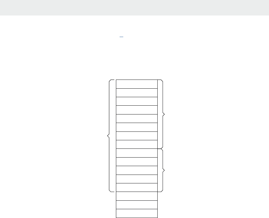
A stack is a conguous block of memory that is accessed in LIFO (last in, rst out) fashion. Data is
added to the top of the stack using a ‘push’ operaon and taken from the top of stack using a ‘pop’
operaon. Stacks are used to store temporary data, and they are commonly used to handle funcon
calls. Most computer architectures include at least a register that is usually reserved for the stack
pointer (e.g., as we have seen the Arm processor has a dedicated ‘SP’ register) as well as ‘PUSH’ and
‘POP’ instrucons to access the stack. In our model, we will implement the stack as part of the RAM
memory, and we dene the push and pop instrucons as in the Arm instrucon set, for example:
Chapter 1 | A Memory-centric system model

Operang Systems Foundaons with Linux on the Raspberry Pi
12
Lisng 1.4.1: Example stack instrucons Python
1 push_pop=[
2 [PUSH,R1],
3 [POP,R2]
4 ]
would push the content of R1 onto the stack and then pop it into R2. The PUSH and POP instrucons
are encoded similar to the LDR and STR memory operaons. We extend the executeInstrucon
denion to support the stack with the following funcons:
Lisng 1.4.2: Push/pop implementaon Python
1 def doPush(registers,systemState,args):
2 sptr = registers[SP]
3 (r1,_,_)=args
4 systemState[sptr]=registers[r1]
5 registers[SP]+=1
6 return (registers,systemState)
7
8 def doPop(registers,systemState,args):
9 sptr = registers[SP]
10 (r1,_,_)=args
11 registers[r1] = systemState[sptr]
12 registers[SP]-=1
13 return (registers,systemState)
1.4.2 Subroune calls
One of the main reasons for having a stack is so that the processor can handle subroune calls, and
in parcular, subrounes that call other subrounes or call themselves (recursive call). This is because
whenever we call a subroune, the code in the subroune will overwrite the register le, so we need
to store the registers somewhere before we call a subroune.
To support this mechanism, most processors have instrucons to change the control ow: a rst
instrucon, the call instrucon changes the program counter to the locaon of the subroune to be called.
A second instrucon, the return instrucon, returns the locaon aer the subroune call instrucon.
These instrucons can use either the stack or a dedicated register to save the program counter.
In the Arm 32-bit instrucon set the call and return instrucons are usually implemented using BL and
BX; the Arm convenon is to store the return address in the link register LR, and we will use the same
convenon in our model. We extend the executeInstrucon denion to support subroune call and
return as follows:
Lisng 1.4.3: Call/return implementaon Python
1 def doCall(registers,args):
2 pctr = registers[PC]
3 (_,sraddr,_)=args
4 registers[LR] = pctr
5 registers[PC]=sraddr

13
6 return registers
7
8 def doReturn(registers,args):
9 lreg = registers[LR]
10 registers[PC]=lreg
11 return registers
1.4.3 Interrupt handling
Now let’s extend the processor model to support interrupts. When the processor receives an interrupt
request, it must take some specic acons. These acons are simply special small programs called
interrupt handlers or interrupt service rounes (ISR). The processor uses a region of the main memory
called the interrupt vector table (IVT) to link the interrupt requests to interrupt handlers.
How does the processor handle interrupts? On every clock ck (i.e., on every call to processorAcon
in our model), if an interrupt was raised, the processor has to run the corresponding ISR. In our model,
this means the processor needs to inspect irqs, get the corresponding ISR from the ivt (which in our
model is a slice of the systemState array), and execute it. So in fact, the call to the ISR is a normal
subroune call, but one that does not have a corresponding CALL instrucon in the code. Before
execung the ISR, the processor typically stores some register values on the stack, e.g., the Arm
Cortex-M3 stores R0-R3, R12, PC, and LR [5]. According to the Arm Architecture Procedure Call
Standard [6], the called subroune is responsible for storing R4-R11. In our simple model, we only
store the PC, extending it to support the AAPCS is a trivial exercise.
Lisng 1.4.4: Interrupt handling Python
1 def checkIrqs(registers,ivt,irqs):
2 idx=0
3 for irq in irqs:
4 if irq :
5 # Save the program counter in the link register
6 registers[LR] = registers[PC]
7 # Set program counter to ISR start address
8 registers[PC]=ivt[idx]
9 # Clear the interrupt request
10 irqs[idx]=False
11 break
12 idx+=1
13 return (registers,irqs)
1.4.4 Direct memory access
Another important component of a modern processor-based system is support for Direct Memory Access
(DMA). This is a mechanism that allows peripherals to transfer data directly into the main memory without
going through the processor registers. In Arm systems, the DMA controller unit is typically a peripheral
(e.g., the PrimeCell DMA Controller), so we will implement our DMA model as a peripheral as well.
The principle of a DMA transfer is that the CPU iniates the transfer by wring to the DMA unit’s
registers, then runs other instrucons while the transfer is in progress, and nally receives an interrupt
from the DMA controller when the transfer is done.
Chapter 1 | A Memory-centric system model

Operang Systems Foundaons with Linux on the Raspberry Pi
14
Typically, a DMA transfer is a transfer of a large block of data, which would otherwise keep the
processor occupied for a long me. In our simple model, the DMA controller has four registers:
Source Address Register (DSR)
Desnaon Address Register (DDR)
Counter (DCO)
Control Register (DCR)
This peripheral is dierent from the others in our model because it can manipulate the enre system
state. In a way, we can view a DMA controller as a special type of processor that only performs
memory transfer operaons. The model implementaon is:
Lisng 1.4.5: DMA model Python
1 def dmaAction(systemState):
2 dmaIrq=0
3 # DMA is the start of the address space
4 # DCR values: 1 = do transfer, 0 = idle
5 if systemState[DMA+DCR]!=0:
6 if systemState[DMA+DCO]!=0:
7 ctr = systemState[DMA+DCO]
8 to_addr = systemState[DMA+DDR]+ctr
9 from_addr = systemState[DMA+DSR]+ctr
10 systemState[to_addr] = systemState[from_addr]
11 systemState[DMA+DCO]=-1
12 systemState[DMA+DCR]=0
13 dmaIrq=1
14 return (systemState,dmaIrq)
To iniate a memory transfer using the DMA controller, the processor writes the source and desnaon
addresses to DSR and DDR, and the size of the transfer to DCO (the ‘counter’). Then the status is set to
1 in the DCR. The DMA controller then starts the transfer and decrements the counter for every word
transferred. When the counter reaches zero, an interrupt is raised (count-zero interrupt).
1.4.5 Complete cycle-based processor model
By including this interrupt support, the complete cycle-based processor model now becomes:
Lisng 1.4.6: Complete cycle-based processor model Python
1 def processorAction(systemState,irqs,registers):
2 ivt = systemState[IVT:IVTsz]
3 # Check for interrupts
4 (registers,irqs)=checkIrqs(registers,ivt,irqs)
5 # Fetch the instruction
6 ir = fetchInstruction(registers,systemState)
7 # Decode the instruction
8 (instr,args) = decodeInstruction(ir)
9 # Execute the instruction
10 (registers,systemState)= executeInstruction(instr,args,registers,systemState)
11 return (systemState,irqs,registers)

15
1.4.6 Caching
In an actual system, accessing DRAM memory requires many clock cycles. To limit the me spent in
waing for memory access, processors have a cache, a small but fast memory. For every memory read
operaon, rst the processor checks if the data is present in the cache, and if so (this is called a ‘cache
hit’) it uses that data rather than accessing the DRAM. Otherwise (‘cache miss’) it will fetch the data
from memory and store it in the cache.
For a single-core processor, memory write operaons are treated in the same way. Real-life caches are very
complicated and will be discussed in more detail in Chapters 3 ‘Hardware architecture’ and 6 ‘Memory
management’. Here we will create a simple conceptual model of a cache to illustrate the key points.
First of all, as a cache is limited in size, how do we store porons of the DRAM content in it? Like the
other memories, we will model the storage part of the cache as an array of xed size. So if we want to
store some data in the cache, we nd a free locaon and copy the data into it. At some point, the data
will be removed from the cache, freeing up this locaon. So we need a data structure, e.g., a stack to
keep track of the free locaons.
So what happens when the cache is full (so the stack is empty)? We need to free up space by evicng data
from the cache. As we will see in Chapter 6 ‘Memory management’, there are several dierent policies
to do this. The simplest one (but certainly not the best one) is to evict data from the most recently used
locaon because all it requires is that we keep track of that single locaon. When we evict data from the
cache, it needs to be wrien back to the DRAM memory. Conversely, the data that we put into the cache
was read from an address locaon in the DRAM memory. Therefore the cache must not only keep track
of the data but also of its original address. In other words, we need a lookup between the address in the
DRAM and the corresponding address in the cache. In Python, we can use a diconary for this, a data
structure that associates keys with values. A cache which behaves like a diconary – in that it allows us to
store any memory address at any cache locaon – is called ‘fully associave’.
In Python, we can write such a cache model as follows:
Lisng 1.4.7: Cache model: inializaon and helper funcons Python
1 # Initialise the cache
2 def init_cache():
3 # Cache of size CACHE_SZ
4 cache_storage=[]
5 location_stack_storage=range(0,CACHE_SZ)
6 location_stack_ptr=CACHE_SZ-1
7 last_used_loc = location_stack[location_stack_ptr]
8 location_stack = (location_stack_storage,location_stack_ptr,last_used_loc)
9 address_to_cache_loc={}
10 cache_loc_to_address={}
11 cache_lookup=(address_to_cache_loc,cache_loc_to_address)
12 cache = (cache_storage, address_to_cache_loc,cache_loc_to_address,location_stac
13 return cache
14
15 # Some helper functions
16 def get_next_free_location(location_stack):
17 (location_stack_storage,location_stack_ptr,last_used_loc) = location_stack
18 loc = location_stack_storage[location_stack_ptr]
19 location_stack_ptr-=1
Chapter 1 | A Memory-centric system model

Operang Systems Foundaons with Linux on the Raspberry Pi
16
20 location_stack = (location_stack_storage,location_stack_ptr,last_used_loc)
21 return (location,location_stack)
22
23 def evict_location(location_stack):
24 (location_stack_storage,location_stack_ptr,last_used_loc) = location_stack
25 location_stack_ptr+=1
26 location_stack[location_stack_ptr] = last_used
27 location_stack = (location_stack_storage,location_stack_ptr,last_used_loc)
28 return location_stack
29
30 def cache_is_full(location_stack_ptr):
31 if location_stack_ptr==0
32 return True
33 else
34 return False
Lisng 1.4.8: Cache model: cache read and write funcons Python
1 def write_data_to_cache(memory, address, cache):
2 (cache_storage, address_to_cache_loc,cache_loc_to_address, location_stack) = cache
3 (location_stack_storage,location_stack_ptr,last_used_loc) = location_stack
4 # If the cache was full, evict rst
5 if cache_is_full(location_stack_ptr):
6 location_stack = evict_location(location_stack)
7 evicted_address = cache_loc_to_address[last_used]
8 memory[evicted_address]=cache_storage[last_used]
9 # Get a free location.
10 (loc,location_stack) = get_next_free_location(location_stack)
11 # Get the DRAM content and write it to the cache storage
12 data = memory[address]
13 cache_storage[loc] = data
14 # Update the lookup table and the last used location
15 address_to_cache_loc[address]=loc
16 cache_loc_to_address[loc] = address
17 last_used=loc
18 location_stack = (location_stack_storage,location_stack_ptr,last_used_loc)
19 cache = (cache_storage,address_to_cache_loc,cache_loc_to_address,location_stack)
20 return (memory,cache)
21
22 def read_data_from_cache(memory,address,cache):
23 (cache_storage, address_to_cache_loc,cache_loc_to_address,location_stack) = cache
24 location_stack = evict_location(location_stack)
25 # If the data is not yet in the cache, fetch it from the DRAM
26 # Note this may result in eviction, which could modify the memory
27 if address not in address_to_cache_loc:
28 (memory, cache) = write_data_to_cache(memory,address,cache):
29 # Get the data from the cache
30 loc = address_to_cache_loc[address]
31 data = cache_storage[loc]
32 cache = (cache_storage, address_to_cache_loc,cache_loc_to_address, location_stack)
33 return (data,memory,cache)
The problem with the above model is that for a cache of a given size, we need a locaon stack and two
lookup tables of the same size. This requires a lot of silicon. Therefore, in pracce, the cache will not
simply fetch the content of a single memory address, but a conguous block of memory called a cache
line. For example, the Arm Cortex-A53 has a 64-byte cache line. Assuming that our memory stores 32-
bit words, then the size of the locaon stack and lookup tables is 16x smaller than the actual cache size.

17
There is another reason for the use of cache lines: when a given address is accessed, subsequent
memory accesses are frequently to neighboring addresses. So fetching an enre cache line on a cache
miss tends to reduce the number of subsequent cache misses. Adapng our model to use cache lines
is straighorward:
Lisng 1.4.9: Cache model with cache lines Python
1 # Initialise the cache
2 def init_cache():
3 # Cache of size CACHE_SZ, cache line = 64 bytes = 16 words
4 cache_storage=[[0]*16]*(CACHE_SZ/16)
5 location_stack_storage=range(0,CACHE_SZ/16)
6 location_stack_ptr=(CACHE_SZ/16)-1
7 last_used_loc = location_stack[location_stack_ptr]
8 location_stack = (location_stack_storage,location_stack_ptr,last_used_loc)
9 address_to_cache_loc={}
10 cache_loc_to_address={}
11 cache_lookup=(address_to_cache_loc,cache_loc_to_address)
12 cache = (cache_storage,address_to_cache_loc,cache_loc_to_address,location_stack)
13 return cache
14
15 # The helper functions remain the same
16
17 def write_data_to_cache(memory,address,cache):
18 (cache_storage, address_to_cache_loc,cache_loc_to_address,location_stack) = cache
19 (location_stack_storage,location_stack_ptr,last_used_loc) = location_stack
20 # If the cache was full, evict rst
21 if cache_is_full(location_stack_ptr):
22 location_stack = evict_location(location_stack)
23 evicted_address = cache_loc_to_address[last_used]
24 cache_line = cache_storage[last_used]
25 for i in range(0,16):
26 data = cache_line[i]
27 memory[(evicted_address<<4) + i]=data
28 # Get a free location.
29 (loc,location_stack) = get_next_free_location(location_stack)
30 # Get the DRAM content and write it to the cache storage
31 cache_line = []
32 for i in range(0,16):
33 cache_line.append(memory[((address>>4)<<4)+i]
34 cache_storage[loc] = cache_line
35 # Update the lookup table and the last used location
36 address_to_cache_loc[address>>4]=loc
37 cache_loc_to_address[loc] = address>>4
38 last_used=loc
39 location_stack = (location_stack_storage,location_stack_ptr,last_used_loc)
40 cache = (cache_storage,address_to_cache_loc,cache_loc_to_address,location_stack)
41 return (memory,cache)
42
43 def read_data_from_cache(memory,address,cache):
44 (cache_storage,address_to_cache_loc,cache_loc_to_address,location_stack) = cache
45 location_stack = evict_location(location_stack)
46 # If the data is not yet in the cache, fetch it from the DRAM
47 # Note this may result in eviction, which could modify the memory
48 if address not in address_to_cache_loc:
49 (memory,cache) = write_data_to_cache(memory,address,cache):
50 # Get the data from the cache
51 loc = address_to_cache_loc[address>>4]
52 cache_line = cache_storage[loc]
53 data = cache_line[addres & 0xF]
54 cache = (cache_storage,address_to_cache_loc,cache_loc_to_address,location_stack)
55 return (data,memory,cache)
Chapter 1 | A Memory-centric system model

Operang Systems Foundaons with Linux on the Raspberry Pi
18
The only complicaon in the cache line-based model is that we need to manipulate the memory
address to determine the start of the cache line and the locaon of the data inside the cache line. Do
this using bit shi and bit mask operaons: the rst 4bits of the address idenfy the posion of the
data in the cache line. We don’t need to store these bits in the lookup tables of the cache because the
cache stores only whole cache lines. In other words, from the perspecve of the cache, the memory
consists of cache lines rather than individual locaons. So we have the following formulas:
data_position_in_cache line = address & 0xF
cache_line_address = address >> 4
address = (cache_line_address << 4) + data_position_in_cache line
1.4.7 Running a program on the processor
The processor model is complete and can run arbitrary programs. For example, the following program
generates the rst 10 Fibonacci numbers greater than 1 and writes them to main memory:
Lisng 1.4.10: Fibonacci code Python
1 b_prog=[
2 [SET,R1,1],
3 [SET,R2,1],
4 [SET,R3,0],
5 [SET,R4,10],
6 [SET,R5,1],
7 (‘loop’,[ADD,R3,R1,R2]),
8 [MOV,R1,R2],
9 [MOV,R2,R3],
10 [SUB,R4,R4,R5],
11 [STR,R3,R4],
12 [CBNZ,R4,’loop’],
13 [WFI]
14 ]
Note: the encodeProgram funcon from abstract_model_encoder.py supports strings as labels for
instrucons as shown above. Similar to Arm assembly language, the instrucons CBZ, CBNZ, ADR, BL,
and B actually take labels rather than explicit addresses.
To run this program, we need to encode it, load it into memory, and ensure that the program counter
points to the start of code in the memory:
Lisng 1.4.11: Running a program on the processor Python
1 # Encode the program
2 b_iws=encodeProgram(b_prog)
3
4 # Write the program to RAM memory
5 pc=0
6 for iw inb_iws:
7 ramState[CODE+pc] = iw
8 pc+=1
9
10 # Initialise the processor state
11 registers[PC]=CODE

19
12
13 # Run the system for a given number of cycles
14 MAX_NCYCLES=50
15 for ncycles in range(1,MAX_NCYCLES):
16 # Run the peripheral actions
17 (kbdState,kbdIrq)=kbdAction(kbdState)
18 (nicState,nicIrq)=nicAction(nicState)
19 (ssdState,ssdIrq)=ssdAction(ssdState)
20 (gpuState,gpuIrq)=gpuAction(gpuState)
21 (systemState,dmaIrq)=dmaAction(systemState)
22
23 # The RAM does not have any action,
24 # it is just a slice of the full address space
25 ramState=systemState[0:MEMTOP]
26 # Collect the IRQs
27 irqs=[kbdIrq,nicIrq,ssdIrq,gpuIrq,dmaIrq]
28 # Compose the system state
29 systemState = ramState+timerState+kbdState+nicState+ssdState+gpuState+dmaState
30 # Run the processor action
31 (systemState,irqs,registers) = processorAction(systemState,irqs,registers)
32
33 # Print the portion of memory that holds the results
34 print(systemState[0:10])
1.4.8 High-level instrucons
The model introduced in the previous secon is cycle-based, i.e., it models all acons and state
changes on a cycle-by-cycle, instrucon-by-instrucon basis. To simplify the explanaons in what
follows and to speed up the execuon of the model code, we add support for direct execuon of high-
level Python code using the HLI instrucon. This allows us to work at a higher level of abstracon,
while sll preserving the low-level features of the system that are used by the operang system.
The previous model required us to write individual instrucons and encode them. The HLI
instrucon allows us to use Python funcons that will replace groups of instrucons, as follows:
Lisng 1.4.12: Mul- instrucon acon Python
1 def multi_instruction_action( systemState,registers ):
2 .... (arbitrary Python code) ...
3 return ( systemState,registers )
4
5 hli_prog = [...,
6 [HLI,multi_instruction_action],
7 ...
8 ]
To execute such funcons in the processor, we add the doHLI funcon to the executeInstrucion code:
Lisng 1.4.13: Adapng push for high-level instrucons Python
1 def doHLI(registers,systemState,args)
2 (hl_instr,_,_)=args
3 (systemState,registers) = hl_instr(systemState,registers)
4 return (registers,systemState)
Chapter 1 | A Memory-centric system model

Operang Systems Foundaons with Linux on the Raspberry Pi
20
To illustrate the approach, the Fibonacci example from the previous secon could become a single HLI
instrucon:
Lisng 1.4.14: Fibonacci with high-level instrucons Python
1 def b_hl( systemState,registers ):
2 (r1,r2,r4)=(1,1,10)
3 while r4!=0:
4 r3=r1+r2
5 r1=r2
6 r2=r3
7 r4-=1
8 systemState[r4]=r3
9 registers[1:5]=[r1,r2,r3,r4]
10 return ( systemState,registers )
The key point is that the funcons manipulate the system state and registers in the same way as the
individual instrucons did.
1.5 Basic operang system concepts
In this secon, we use the abstract system model to introduce a number of fundamental operang
system concepts that will be discussed in detail in the following chapters.
1.5.1 Tasks and concurrency
One of the main tasks of an operang system is to support mulple tasks at the same me
(‘concurrently’). If there is only one processor, it means that the code that implements these tasks must
me-share the processor. Let us assume that we have two programs in memory and we want to run
them concurrently so that each running program is a single task, Task 1 and Task 2.
We have seen in Secon 1.4.7 how we run a program: set the program counter to the starng address,
then the fetch-decode-execute cycle will execute each instrucon on subsequent clock cks unl the
program is nished.
Now we want to run two programs at the same me. Therefore, we will need a mechanism to run
instrucons of each program alternangly. This mechanism translates to managing the state. As we
have seen before, the state of a running program consists in principle of the complete system state.
In pracce, each program should have its own secon of memory, as we don’t want one program to
modify the memory of another program.
We start, therefore, by assuming that when the program code is loaded into memory, it is part of
a region of memory that the program is allowed to use when it is running. We will see in Chapter 6
‘Memory management’ that this is indeed the case in Linux. As shown in Figure 1.3, this region (called
‘user space’) contains the program code, the stack for the program and the random-access memory
for the program, commonly known as the ‘heap’. Typically, each task gets a xed amount of memory
allocated to it, and in the code, this memory is referenced relave to the program counter.
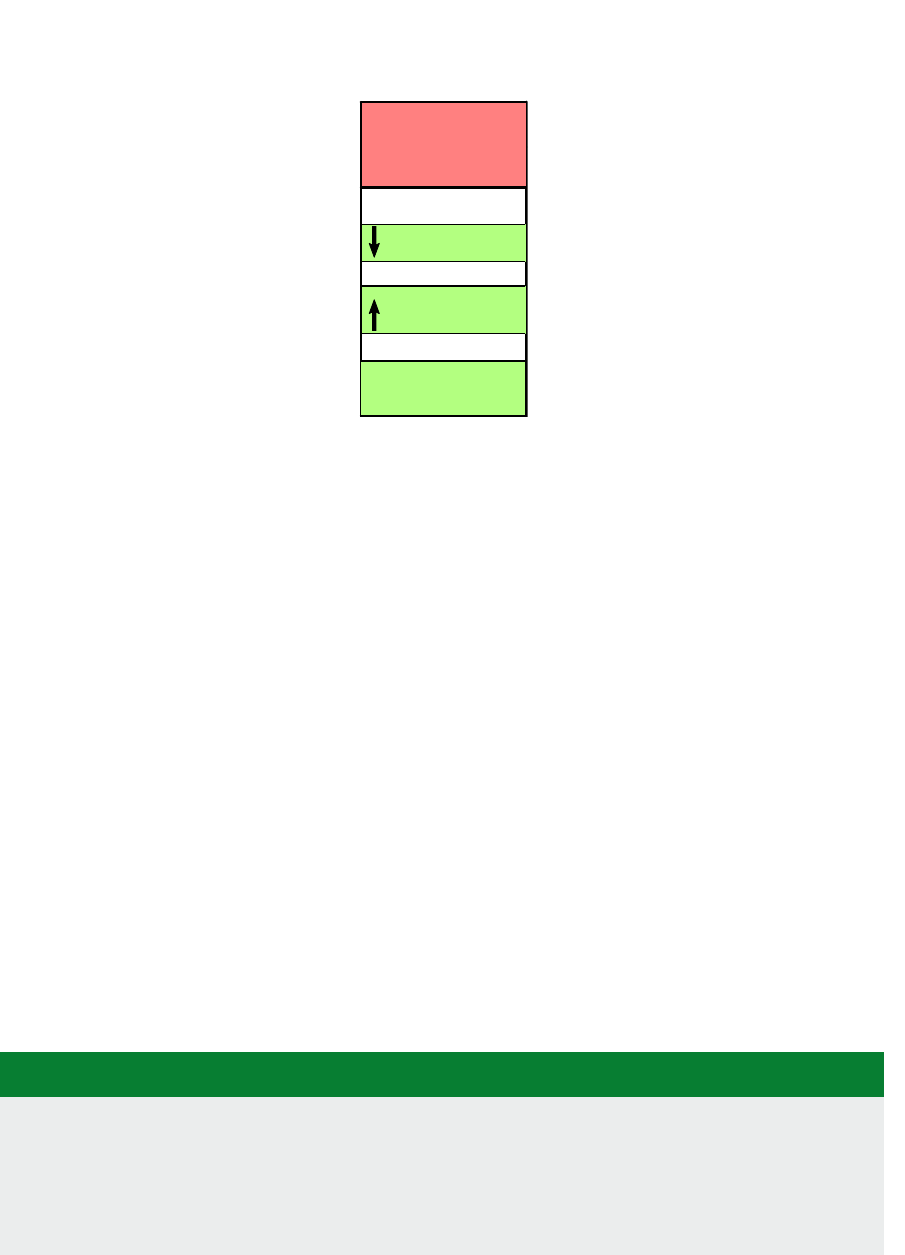
21
Figure 1.3: Task memory space (Linux).
1.5.2 The register le
However, as we have seen, the processor also has some state, namely the register le. So if we want
to run two tasks alternately, we need to ensure that the register le contains the correct state for each
task. So conceptually, we can store a snapshot of the register le contents for Task 1, then load the
previous snapshot of the register le contents for Task 2.
1.5.3 Time slicing and scheduling
So how can we make two tasks alternate? The code to do this will be the core of our Operang System
kernel and is called a ‘task scheduler’ or scheduler for short. Let’s assume we will simply alternate two
(or more) tasks for xed amounts of me (this is called ‘round-robin scheduling’). For example, on the
Raspberry Pi 3, the Linux real-me scheduler uses an interval (also called ‘me slice’ or ‘quantum’) of
10 ms. For comparison, the average duraon of an eye blink is 100 ms. Note that at a typical clock
speed of 1 GHz, this means a task can execute 10 million (single-cycle) instrucons in this me.
The duraon of a me slice is controlled by a system mer. As we have seen before, a mer can be
congured to re periodically, so in our case, the system mer will raise an interrupt request every
10 ms. On receiving this request, the processor will execute the corresponding Interrupt Service
Roune (ISR). It is this ISR that will take care of the me slicing; in other words, the interrupt service
roune is actually our operang system kernel.
In the Python model, the mer peripheral has a register to store the interval and a control register.
We can set the mer as follows:
Lisng 1.5.1: Timer Python
1 # Set timer to periodic with 100-ticks interval
2 set_timer=[
3 [SET,R1,100],
4 [SET,R2,100], # start periodic timer
5 [STR,R1,TIMER],
6 [STR,R2,TIMER+1]
7 ]
program code
stack
kernel space
0 GB
3 GB
4 GB
user space
heap
Chapter 1 | A Memory-centric system model

Operang Systems Foundaons with Linux on the Raspberry Pi
22
On running this program, the mer will re every 100 clock cks and raise an interrupt request. Let’s
have a look at the interrupt handler. What should this roune do to achieve me slicing between two
tasks? Let’s assume Task 1 has been running and we now want to run Task 2.
First, save the register le for Task 1, we do this by pushing all register contents onto the stack.
(If you spot an issue here, well done! We’ll get back to this in Secon 1.5.4.)
Then determine which task has to be run next (i.e., Task 2). We can idenfy each task using a small
integer (the ‘task idener’) that we store in the memory accessible by the kernel. We load the task
idener for Task 2 into a register and update the memory with the task idener for the next task
(in our case, again Task 1).
We now move the register le of Task 1 from the stack to kernel memory. In pracce, the kernel
uses a special data structure, the Task Control Block (TCB), for this purpose.
Now we can read the register le contents for Task 2 from its TCB. Again, we have to do this via the
stack (why?).
Once this is done, Task 2 will start running from the locaon indicated by PC and run unl the next
mer interrupt.
We can express this sequence of acons in high-level Python code for our processor model:
Lisng 1.5.2: Time slicing model Python
1 def time_slice(systemState,registers ):
2 # Push registers onto the stack
3 for r in range(0,16):
4 systemState[registers[MSP]]]=registers[r]
5 registers[MSP]+=1
6 # Get next task
7 pid1 = systemState[PID] # 0 or 1
8 pid2 = 1-pid1
9 systemState[PID]=pid2
10 tcb1= TCB_OFFSET+pid1*TCB_SZ
11 tcb2= TCB_OFFSET+pid2*TCB_SZ
12 # Pop registers from stack and store to tcb1
13 # We use r0 to show that in actual code we’d need to read into a tempory register
14 for r in range(0,16):
15 r0=systemState[registers[MSP]]
16 systemState[tcb1+r]=r0
17 registers[MSP]-=1
18 # Push registers for Task 2 from tcb2 onto stack
19 for r in range(0,16):
20 r0=systemState[tcb2+r]
21 systemState[registers[MSP]]=r0
22 registers[MSP]+=1
23 # Pop registers for Task 2 from stack
24 for r in range(0,16):
25 registers[r]=systemState[registers[MSP]]
26 registers[MSP]-=1
This code is a minimal example of a round-robin scheduler for two tasks.

23
You can already try and answer these quesons by thinking about how you would address these issues.
1.5.4 Privileges
In Secon 1.5.3, we hinted at a potenal issue with the stack. The problem is that ‘pushing onto the
stack’ means modifying the stack pointer SP. So how can we preserve the stack pointer of the current
task? The short answer for the Arm processor is that it has two stack pointers, one for user space task
stacks (PSP) and one for the kernel stack (MSP). User tasks cannot access the kernel stack pointer; the
kernel code can select between the two using the MRS and MSR instrucon.
This raises the topic of privileges: clearly if the kernel code can access more registers than the user
task code, the kernel code is privileged. This is an essenal security feature of any operang system
because, without privileges, a userspace task code could modify the kernel code or other task code.
We will discuss this in more detail in Chapter 4, ‘Process management’. For the moment, it is sucient
to know that in the Arm Cortex-M3 there are two privilege levels
4
, ‘Unprivileged’ and ‘Privileged’; in
Unprivileged mode the soware has limited access to the MSR and MRS instrucons which allow
access to special registers, and cannot use the CPS instrucon which allows us to change the privilege
level. For further restricons, see [2].
1.5.5 Memory management
So far, we have assumed that tasks already reside in memory. In pracce, the OS will have to load
the program code into memory. To do so, the OS must nd a sucient amount of memory for
both the program code and the memory required by the program. It would clearly not be praccal
if the program were to use absolute memory addresses: this would mean that the compiler (or the
programmer) would need to know in advance where the program would reside in memory. This would
be very inexible. Therefore, program code will use relave addressing, e.g., relave to the value of
the program counter. The OS will set the PC to the starng address of the code in memory.
However, relave addressing does not solve all problems. The main queson is how to allocate space
in memory for the processes. Inially, we could of course simply ll up the memory, as shown in
Figure 1.4. But what happens with the memory of nished tasks? The OS should, of course, reuse it,
but it could only do so if a new task does not use any more memory than one of the nished tasks.
Again, this would be very restricve.
The commonly used soluon to this problem is to introduce the concept of a logical address space.
This is a conguous address space allocated to a process. The physical addresses that correspond to
this logical address space do not have to be conguous. The operang system is responsible for the
translaon between the logical and physical address spaces. What this involves is explained in detail
in Chapter 6, ‘Memory management’, but you can already think of ways to organize non-conguous
blocks of physical memory of varying size into a logical conguous space. Apart from address
translaon, the OS also must ensure that a process cannot access the memory space of another
process: this is called memory protecon. Typically, this involves checking a logical address against
the upper and a lower bound of the process logical address space. Because this is a very common
4
In more advanced processors such as the Arm Cortex-A53, there are 4 levels of privilege, called ‘Excepon Levels’ (EL) and numbered EL0-EL3. The userspace tasks run
in EL0, the OS kernel in EL1.
Chapter 1 | A Memory-centric system model
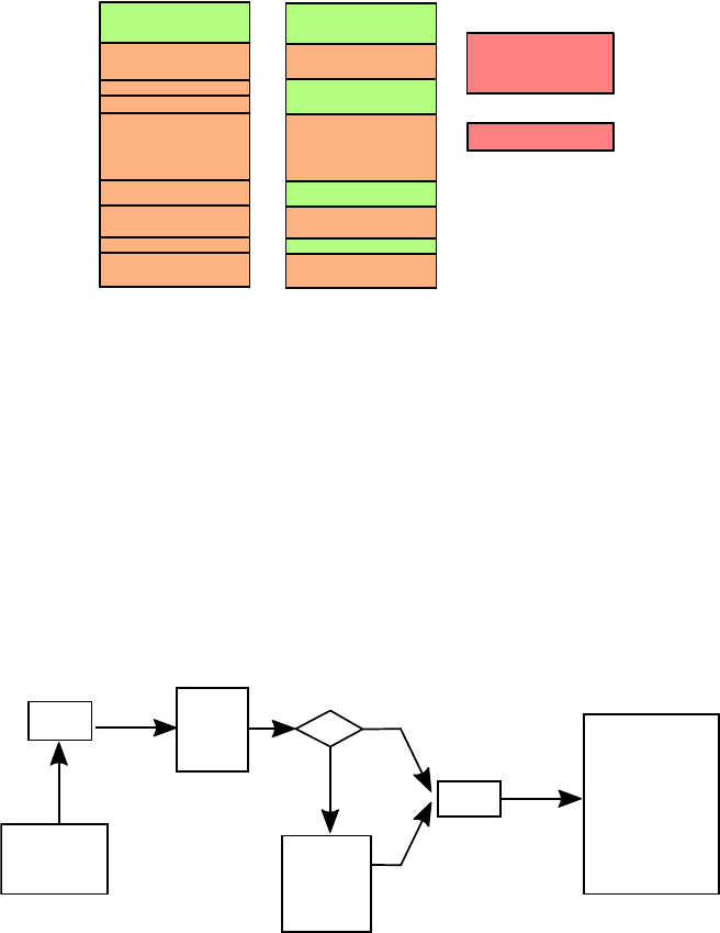
Operang Systems Foundaons with Linux on the Raspberry Pi
24
operaon, there is usually hardware support for it in the form of a Memory Protecon Unit (MPU) in
low-end processors such as the Cortex-M3 or as part of a more elaborate Memory Management Unit
(MMU) in processors such as the Cortex-A53.
Figure 1.4: Problem with conguous memory allocaon.
1.5.6 Translaon look-aside buer (TLB)
The MMU can be implemented as a peripheral as we have done for the DMA unit above, but we
will defer this to the in-depth discussion of memory management provided in Chapter 6. However,
we want to introduce one parcular part of the MMU, a special type of cache called the translaon
look-aside buer (TLB). The translaon from logical to physical addresses is quite me-consuming, and
therefore, the MMU uses the TLB to keep track of recently used translaons (Figure 1.5). Unlike the
memory cache, which contains the data stored in the memory, the TLB contains the physical address
corresponding to a logical address.
Figure 1.5: Logical to physical address translaon with translaon look-aside buer (TLB).
The same consideraons which lead us to use cache lines lead to a similar approach to reducing the
memory space: we divide both the logical and physical memory into chunks of a xed size (which we
call respecvely pages and frames), and we store the starng addresses of those chunks in the TLB,
rather than individual addresses. The posion inside the page is calculated in quite the same way as
the posion in a cache line, using a xed number of LSBs. Typically, pages in Linux are 4KB; dierent
sizes are possible; see Chapter 3 and Chapter 7. The TLB diers from the cache in that a miss does
Logical
address
Physical
address
hit
miss
TLB
Page
table
Physical
memory
CPU
Initial memory use
(green = empty)
Memory use after tasks
2,4,6 and 7 have finished
task 9
task 10
Where to allocate
tasks 9 and 10?
task 2
task 1
task 3
task 5
task 4
task 7
task 6
task 8
task 1
task 3
task 5
task 8

25
not result in a fetch from memory but in a lookup of the physical address in what is called the Page
Table; also, writes to the TLB only happen on a miss. However, the similarity between the cache and
TLB serves allows us to explain the main points of memory management without the need to know
anything about how the actual Page Table works.
1.6 Exercises and quesons
1.6.1 Task scheduling
1. Create a scheduler for a single task in Python. You can use the above code and the Fibonacci
example, or you can write your own code.
2. Extend the me_slice funcon and the memory layout to support a larger number (NTASKS) tasks.
1.6.2 TLB model
1. Create a TLB model in Python, starng from the cache model code in Secon 1.4.6.
2. Given the concept of logical and physical address spaces and the idea of pages, propose a data
structure that allows the OS to allocate non-conguous blocks of physical memory to a process
as a conguous logical address space. Discuss the pros and cons of your proposed data structure.
3. Assuming 4GB of memory divided into 4KB-size pages, and assuming that the page table lookup
is 100x slower than the TLB lookup. What should be the hit rate of the TLB to have an average
lookup me of twice the TLB lookup me? What would the TLB size have to be?
1.6.3 Modeling the system
1. In a physical system, all acons in the above model take place in parallel. What eect does this have
on the model?
2. Suppose you have to design the peripheral for a keyboard which has no locking keys nor modier
keys. What would be the state and which events would raise interrupts?
1.6.4 Bare-bones processor model
1. The LDR and STR instrucons work on memory addresses. In principle, there is nothing that
stops two programs from using the same memory addresses, but this is, of course, in general, not
desirable. What could we do to avoid this?
2. Can you think of features that our bare bones processor is missing?
1.6.5 Advanced processor model
1. If the processor has mulple cores that can execute tasks in parallel, what would need to change to
the processor model?
2. Can you see any issues with the cache if every core would have its own cache? What if they share
a single cache?
1.6.6 Basic operang system concepts
The explanaon in Secon 1.5 omits a lot of detail and raises several quesons, which will be
answered in the later chapters. For example:
What happens if there are more than 2 running tasks?
How does a user start a task?
Chapter 1 | A Memory-centric system model

Operang Systems Foundaons with Linux on the Raspberry Pi
26
How does the OS load programs from disk into in memory?
How does the OS ensure that programs can only access their own memory?
What about sharing of peripherals?
What happens when a task is nished?
The issues of privileges and memory management are discussed in more detail in Chapters 5 and 6.
The model presented so far raises several quesons:
What does it involve to guarantee memory protecon? For example, how could the OS know the
bounds of the logical address space of each process?
Is it sucient to provide memory protecon? Should other resources have similar protecons?
What could be the reason that the default page size on Linux is 4KB? What would happen if it was
10x smaller, or 10x larger?
Can you think of scenarios where logical memory is not necessary?
References
[1] Principles of Arm Memory Maps, Arm Ltd, 10 2012, issue C. [Online].
Available: hp://infocenter.arm.com/help/topic/com.arm.doc.den0001c/DEN0001C_principles_of_arm_memory_maps.pdf
[2] Arm
®
Cortex
®
-A53 MPCore Processor – Technical Reference Manual Rev: r0p4, Arm Ltd, 2 2016, revision: r0p4. [Online].
Available: hp://infocenter.arm.com/help/topic/com.arm.doc.ddi0500g/DDI0500G_cortex_a53_trm.pdf
[3] ARM Compiler toolchain Version 5.03 Assembler Reference, Arm Ltd, 1 2013. [Online].
Available: hp://infocenter.arm.com/help/topic/com.arm.doc.dui0489i/DUI0489I_arm_assembler_reference.pdf
[4] A. G. Dean, Embedded Systems Fundamentals with Arm Cortex-M based Microcontrollers: A Praccal Approach.
Arm Educaon Media UK, 2017.
[5] Cortex™-M3 Devices Generic User Guide, Arm Ltd, 12 2010. [Online].
Available: hp://infocenter.arm.com/help/topic/com.arm.doc.dui0552a/DUI0552A_cortex_m3_dgug.pdf
[6] Procedure Call Standard for the Arm Architecture ABI r2.10, Arm Ltd, 2015. [Online].
Available: hps://developer.arm.com/docs/ihi0042/latest/procedure-call-standard-for-the-arm-architecture-abi-2018q4-documentaon

27
Chapter 1 | A Memory-centric system model

Chapter 2
A praccal view
of the Linux system
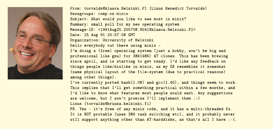
Operang Systems Foundaons with Linux on the Raspberry Pi
30
2.1 Overview
In this chapter, we approach the Linux system from a praccal perspecve, as experienced by users
of the system, in parcular administrators and applicaon programmers rather than kernel or driver
programmers. We rst introduce the essenal concepts and techniques that you need to know in order
to understand the overall system, and then we discuss the system itself from dierent angles: what
is the OS role in boong and inializing the system; what OS knowledge does a system administrator
and systems programmer need. This chapter is not a how-to guide, but rather provides you with the
background knowledge behind how-to guides. It also serves as a roadmap for the rest of the book.
What you will learn
Aer you have studied the material in this chapter, you will be able to:
1. Explain basic operang system concepts: processes, users, les, permissions, and credenals.
2. Analyze the chain of events when boong Linux on the Raspberry Pi.
3. Create a Linux kernel module and build a custom Linux kernel.
4. Discuss the administrator and programmers view on the key operang system concepts covered in
the further chapters.
2.2 Basic concepts
To understand what happens when the system boots and inializes, as well as how the OS aects
the tasks of system administrator and systems programmer, we need to introduce a number of basic
operang system concepts. Most of these apply to any operang system, although the discussion
here is specic to Linux on Arm-based systems. The in-depth discussion of these concepts forms the
subject of the later chapters, so this secon serves as a roadmap for the rest of the book as well.
The original Linux
announcement on
Usenet (1991).
Photo by Krd.

31
2.2.1 Operang system hierarchy
The Linux kernel is only one component of the complete operang system. Figure 2.1 illustrates the
complete Linux system hierarchy. Interfacing between the kernel and the user space applicaons is
the system call interface, a mechanism to allow user space applicaons to interact with the kernel
and hardware. This interface is used by system tools and libraries, and nally by the user applicaons.
The kernel provides funconality such as scheduling, memory management, networking and le
system support, and support for interacng with system hardware via device drivers.
Interfacing between the kernel and the hardware are device drivers and the rmware. In the Linux
system, device drivers interact closely with the kernel, but they are not considered part of the kernel
because depending on the hardware dierent drivers will be needed, and they can be added on the y.
2.2.2 Processes
A process is a running program, i.e., the code for the program and all system resources it uses.
The concept of a process is used for the separaon of code and resources. The OS kernel allocates
memory resources and other resources to a process, and these are private to the process, and
protected from all other processes. The scheduler allocates me for a process to execute. We also use
the term task, which is a bit less strictly dened, and usually relates to scheduling: a task is an amount
of work to be done by a program. We will also see the concept of threads, which are used to indicate
mulple concurrent tasks execung within a single process. In other words, the threads of a process
share its resources. For a process with a single thread of execuon, the terms task and process are
oen used interchangeably.
When a process is created, the OS kernel assigns it a unique idener (called process ID or PID for
short) and creates a corresponding data structure called the Process Control Block or Task Control
Block (in the Linux kernel this data structure is called task_struct). This is the main mechanism the
kernel uses to manage processes.
Figure 2.1: Operang System Hierarchy.
Linux Kernel
Operating System
Firmware
Applications
System Call Interface
VFS
File Systems
Volume Manager
Block Device Int.
Sockets
TCP/UDP
IP
Ethernet
Scheduler
Virtual
Memory
System Libraries
Device Drivers
Clocksource
based http://www.brendangregg.com/linuxperf.html
CC BY-SA Brendan Gregg 2017
System Tools
Chapter 2 | A praccal view of the Linux system
Operang Systems Foundaons with Linux on the Raspberry Pi
32
2.2.3 User space and kernel space
The terms ‘user space’ and ‘kernel space’ are used mainly to indicate process execuon with dierent
privileges. As we have seen in Chapter 1, the kernel code can access all hardware and memory in the system,
but for user processes, the access is very much restricted. When we use the term ‘kernel space,’ we mean
the memory space accessible by the kernel, which is eecvely the complete memory space in the system
1
.
By ‘user space,’ we mean the memory accessible by a user process. Most operang systems support mulple
users, and each user can run mulple processes. Typically, each process gets its own memory space, but
processes belonging to a single user can share memory (in which case we’ll call them threads).
2.2.4 Device tree and ATAGs
The Linux kernel needs informaon about the system on which it runs. Although a kernel binary must be
compiled for a target architecture (e.g., Arm), a kernel binary should be able to run on a wide variety of
plaorms for this architecture. This means that the kernel has to be provided with informaon about the
hardware at boot me, e.g., number of CPUs, amount of memory, locaon of memory, devices and their
locaon in the memory map, etc. The tradional way to do this on Arm systems was using a format called
ATAGs, which provided a data structure in the kernel that would be populated with informaon that the
bootloader provided. A more modern and exible approach is called Device Tree
3
. It denes a format and
syntax to describe system hardware in a Device Tree Source le. A device tree is a tree data structure with
nodes that describe the physical devices in a system. The Device Tree source les can be compiled using
a special compiler into a machine-architecture-independent binary format called Device Tree Blob.
2.2.5 Files and persistent storage
The Linux Informaon Project denes a le as:
A le is a named collecon of related data that appears to the user as a single, conguous block of
informaon and that is retained in storage.
2
In this denion, storage refers to computer devices or media which can retain data for relavely long
periods (e.g., years or decades), such as solid state drives and other types of non-volale memory,
magnec hard disk drives (HDDs), CDROMs and magnec tape, in other words, persistent storage.
This is in contrast with RAM memory, the content of which is retained only temporarily (i.e., only while
in use or while the power supply remains on).
A persistent storage medium (which I will call ‘disk’) such as an SD card, USB memory sck or hard
disk, stores data in a linear fashion with sequenal access. However, in pracce, the disk does not
contain a single array of bytes. Instead, it is organized using parons and le systems. We discuss
these in more detail in Chapter 9, but below is a summary of these concepts.
Paron
A disk can be divided into parons, which means that instead of presenng as a single blob of data,
it presents as several dierent blobs. Parons are logical rather than physical, and the informaon
about how the disk is paroned (i.e., the locaon, size, type, name, and aributes of each paron)
is stored in a paron table. There are several standards for the structure of parons and paron
tables, e.g., GUID Paron Table and MBR.
1
Assuming the system does not run a hypervisor. Otherwise, it is the memory available to the Virtual Machine running the kernel.
2
hp://www.linfo.org/le.html
3
hps://www.devicetree.org/specicaons
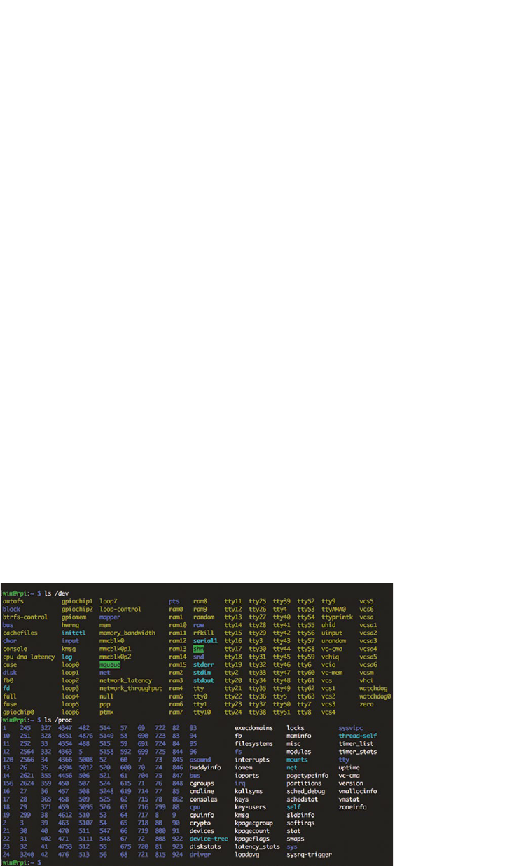
33
File system
Each paron of a disk contains a further system for logical organizaon. The purpose of most le
systems is to provide the le and directory (folder) abstracons. There are a great many dierent
le systems (e.g., fat32, ext4, hfs+, ...) and we will cover the most important ones in Chapter 9. For
the purpose of this chapter, what you need to know is that a le system not only allows to store
informaon in the form of les organized in directories but also informaon about the permissions
of usages for les and directories, as well as mestamp informaon (le creaon, modicaon, etc.).
The informaon in a le system is typically organized as a hierarchical tree of directories, and the directory
at the root of the tree is called the root directory. To use a le system, the kernel performs an operaon
called mounng. As long as a le system has not been mounted, the system can’t access the data on it.
Mounng a le system aaches that le system to a directory (mount point) and makes it available
to the system. The root (/) le system is always mounted. Any other le system can be connected or
disconnected from the root le system at any point in the directory tree.
2.2.6 ‘Everything is a le’
One of the key characteriscs of Linux and other UNIX-like operang systems is the oen-quoted
concept of ‘everything is a le.’ This does not mean that all objects in Linux are les as dened above, but
rather that Linux prefers to treat all objects from which the OS can read data or to which it can write data
using a consistent interface. So it might be more accurate to say ‘everything is a stream of bytes.’ Linux
uses the concept of a le descriptor, an abstract handle used to access an input/output resource (of which
a le is just one type). So one can also say that in Linux, ‘everything is a le descriptor.’
What this means in pracce is that the interface to, e.g., a network card, keyboard or display is
represented as a le in the le system (in the /dev directory); system informaon about both hardware
and soware is available under /proc. For example, Figure 2.2 shows the lisng of /dev and /proc on
the Raspberry Pi. We can see device les represenng memory (ram*), terminals (y*), modem (ppp),
Figure 2.2: Lisng of /dev and /proc on the Raspberry Pi running Raspbian.
Chapter 2 | A praccal view of the Linux system
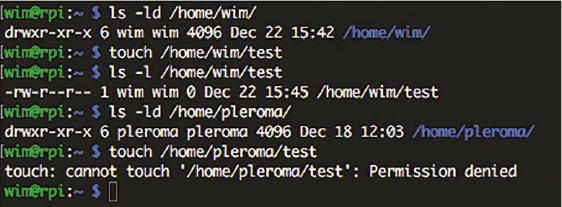
Operang Systems Foundaons with Linux on the Raspberry Pi
34
and many others. In parcular, there is /dev/null which is a special device which discards the
informaon wrien to it, and /dev/zero which returns an endless stream of zero bytes (i.e., 0x00,
so when you try cat /dev/zero you will see nothing. Try cat/dev/zero | hd instead.)
2.2.7 Users
A Linux system is typically a mul-user system. What this means is that it supports another level
of separaon, permissions, and protecon above the level of processes. A user can run and control
mulple processes, each in their own memory space, but with shared access to system resources.
In parcular, the concept of users and permission is ghtly connected with the le system. The le
system permissions for a given user control the access of that user in terms of reading, wring, and
execung les in dierent parts of the le system hierarchy.
Just as the kernel runs in privileged mode to control the user space processes, there is also a need
for a privileged user to control the other users (similar to the ‘Administrator’ on Windows systems).
In Linux, this user is called root
3
and when the system boots, the rst process (init, which has PID=1)
is run as the root user. The init process can create new processes. In fact, in Linux, any process can
create new processes (as explained in more detail in Chapter 4). However, a process owned by the
root user can assign ownership of a created process to another user, whereas processes created by
a non-root user process can only be owned by itself.
2.2.8 Credenals
In Linux, credenals is the term for the set of privileges and permissions associated with any object.
Credenals express, e.g., ownership, capabilies, and security management properes. For example,
for les and processes, the key credenals are the user id and group id. To decide what a certain object
(e.g., a task) can do to another object (e.g., a le), the Linux kernel performs a security calculaon using the
credenals and a set of rules. In pracce, processes executed as root can access all les and other resources
in the system; for a non-root user, le and directory access is determined by a system of permissions on
the les and by the membership of groups: a user can belong to one or more groups of users.
File access permissions can be specied for individual users, groups, and everyone. For example, in
Figure 2.3, we see that the directory /home/wim can be wrien to by user wim in group wim. If we try
to create an (empty) le using the touch command, this succeeds. However, if we try to do the same
in the directory /home/pleroma, owned by user pleroma in group pleroma, we get ‘permission denied’
because only user pleroma has write access to that directory.
Figure 2.3: Example of restricons on le creaon on the Raspberry Pi running Raspbian.
3
For more info about the origin of the name, root see www.linfo.org/root.html
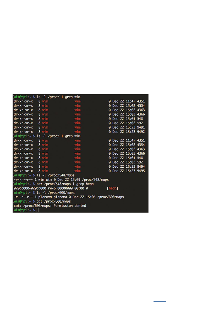
35
Note that because of the ‘everything is a le’ approach, this system of permissions extends in general
to devices, system informaon, etc. However, the actual kernel security policies can restrict access
further. For example, in Figure 2.2, the numbers in the /proc lisng represent currently running
processes by their PID.
To illustrate the connecon between users, permissions, and processes, Figure 2.4 shows how user
wim can list processes in /proc belonging to two dierent non-root users, wim, and pleroma.
The command cat /proc/548/maps prints out the enre memory map for the process with PID
548. The map is quite large, so for this example, only the heap memory allocaon is shown (using
grep heap).
Figure 2.4: Example of restricons on process memory access via /proc on the Raspberry Pi running Raspbian.
However, when we try to do the same with /proc/600/maps, we get ‘Permission denied’ because
the cat process owned by user wim does not have the right to inspect the memory map of a process
owned by another user. This is despite the le permissions allowing read access.
2.2.9 Privileges and user administraon
The system administrator creates user accounts and decides on access to resources using groups
(using tools such as useradd(8), groupadd(8), chgrp(1), etc.). The kernel manages credenals per
process using struct cred which is a eld of the task_struct.
The admin also decides how many resources each user and process gets, e.g., using ulimit.
Resource limits are set in /etc/security/limits.conf and can be changed at runme via the
shell command ulimit. Internally, the ulimit implementaon uses the getrlimit and setrlimit system calls
which modify the kernel struct rlimit in include/uapi/linux/resource.h.
Chapter 2 | A praccal view of the Linux system
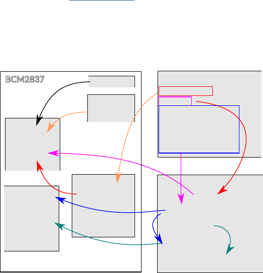
Operang Systems Foundaons with Linux on the Raspberry Pi
36
2.3 Boong Linux on Arm-based systems (Raspberry Pi 3)
In this secon, we discuss the boot process for Linux on the Raspberry Pi 3. The boot sequence of
Linux on Arm-based systems varies signicantly from plaorm to plaorm. The dierences somemes
arise due to the needs of the target market but can also be due to choices made by SoC and plaorm
vendors. The boot sequence discussed here is a specic example to demonstrate what happens on
a parcular plaorm.
This Raspberry Pi 3 (Figure 2.5) runs Raspbian Linux on an Arm Cortex-A53 processor which is part of
the Broadcom BCM2837 System-on-Chip (SoC). This SoC also contains a GPU (Broadcom VideoCore
IV) which shares the RAM with the CPU. The GPU controls the inial stages of the boot process. The
SoC also has a small amount of One Time Programmable (OTP) memory which contains informaon
about the boot mode and a boot ROM with the inial boot code.
Figure 2.5: Boot Process for Raspbian Linux on the Raspberry Pi 3.
2.3.1 Boot process stage 1: Find the bootloader
Stage 1 of the boot process begins with reading the OTP to check which boot modes are enabled.
By default, this is SD card boot, followed by a USB device boot. The code for this stage is stored in the
on-chip ROM. The boot code checks each of the boot sources for a le called bootcode.bin in the
root directory of the rst paron on the storage medium (FAT32 formaed); if it is successful, it will
load the code into the local 128K (L2) cache and jump to its rst instrucon to start Stage 2.
Note: The boot ROM supports GUID paroning and MBR-style paroning.
2.3.2 Boot process stage 2: Enable the SDRAM
Stage 2 is controlled by bootcode.bin, which is closed-source rmware. It enables the SDRAM and
loads Stage 3 (start.elf) from the storage medium into the SDRAM.
OTP
GPU
Arm
Cortex-A53
CPU
SSD
SDRAM
bootcode.bin
L2 cache
ROM
start.elf
Stage 1.a
Stage 1.b
Stage 3.a
Stage 1.c
bootcode.bin
start.elf
[boot code]
Stage 2.b
kernel.img
kernel.img
config.txt
cmdline.txt
bcm2710-rpi-3-b.dtb
bcm2710-rpi-3-b.dtb
Stage 2.a
Stage 4.a
Stage 3.b
[decompressed
kernel code]
Stage 5.a
BCM2837
initramfs.gz
initramfs.gz
[mounted initramfs]
Stage 5.b
Stage 4.b

37
2.3.3 Boot process stage 3: Load the Linux kernel into memory
Stage 3 is controlled by start.elf, which is a closed-source ELF-format binary running on the GPU.
start.elf loads the compressed Linux kernel binary kernel.img and copies it to memory. It reads
cong.txt,cmdline.txt and bcm2710-rpi-3-b.dtb (Device Tree Binary).
The le cong.txt is a text le containing system conguraon parameters which would on
a convenonal PC be edited and stored using a BIOS.
The le cmdline.txt contains the command line arguments to be passed on to the Linux kernel
(e.g., the le system type and locaon of the root le system) using ATAGs, and the .dtb le contains
the Device Tree Blob.
2.3.4 Boot process stage 4: Start the Linux kernel
Stage 4 starts kernel.img on the CPU: releasing reset on the CPU causes it to run from the address
where the kernel.img data was wrien. The kernel runs some Arm-specic code to populate CPU
registers and turn on the cache, then decompresses itself, and runs the decompressed kernel code.
The kernel inializes the MMU using Arm-specic code and then run the rest of the kernel code which
is processor-independent.
2.3.5 Boot process stage 5: Run the processor-independent kernel code
Stage 5 is the processor-independent kernel code. This code consists mainly of inializaon funcons
to set up interrupts, perform further memory conguraon, and load the inial RAM disk initramfs.
This is a complete set of directories that you would nd on a normal root le system and was loaded
into memory by the Stage 3 boot loader. It is copied into kernel space memory and mounted. This
initramfs serves as a temporary root le system in RAM and allows the kernel to fully boot and
perform user-space operaons without having to mount any physical disks.
A single Linux kernel image can run on mulple plaorms with support for a large number of devices/
peripherals. To reduce the overhead of loading and running a kernel binary bloated with features that
aren’t widely used, Linux supports runme loading of components (modules) that are not needed
during early boot. Since the necessary modules needed to interface with peripherals can be part of
the initramfs, the kernel can be very small, but sll, support a large number of possible hardware
conguraons. Aer the kernel is booted, the initramfs root le system is unmounted, and the real
root le system is mounted. Finally, the init funcon is started, which is the rst user-space process.
Aer this, the idle task is started, and the scheduler starts operaon.
2.3.6 Inializaon
Aer the kernel has booted it launches the rst process, called init. This process is the parent of all
other processes. In the Raspbian Linux distribuon that runs on the Raspberry Pi 3, this init is
actually an alias for /lib/systemd/systemd because Raspbian, as a Debian-derived distribuon,
uses systemd as its init system. Other Linux distribuons can have dierent implementaons of init,
e.g., SysV init or upstart.
Chapter 2 | A praccal view of the Linux system

Operang Systems Foundaons with Linux on the Raspberry Pi
38
The systemd process executes several processes to inialize the system: keyboard, hardware drivers, le
systems, network, services. It has a sophiscated system for conguring all the processes under its control
as well as for starng and stopping processes, checking their status, logging, changing privileges, etc.
The systemd process performs many tasks, but the principle is always the same: it starts a process
under the required user name and monitors its state. If the process exits, systemd takes appropriate
acon, e.g., restarng the process or reporng the error that caused it to exit.
2.3.7 Login
One of the systemd responsibilies is running the processes that let users log into the system
(systemd-logind). To login via a terminal (or virtual console), Linux uses two programs: gey and login
(originally, the y in gey meant ‘teletype,’ a precursor to modern terminals). Both run as root.
A basic gey program opens the terminal device, inializes it, prints the login prompt, and waits
for a user name to be entered. When this happens, gey executes the login program, passing it the
user name to log in as. The login program then prompts the user for a password. If the password is
wrong, login simply exits. The systemd process will noce this and spawn another gey process. If the
password is correct, login executes the user’s shell program as that user. From then on, the user can
start processes via the shell.
The reason why there are two separate programs is that both gey and login can be used on their own,
for example, a remote login over SSH does not use a terminal but sll uses login: each new connecon
is handled by a program called sshd that starts a login process.
A graphical login is conceptually not that dierent from the above descripon. The dierence is that
instead of the gey/login programs, a graphical login program called the display manager is run, and
aer authencaon, this program launches the graphical shell.
In Raspbian the display manager is LightDM, and the graphical shell is LXDE (Lightweight X11 Desktop
Environment). Like most Linux distribuons, the graphical desktop environment is based on the X
Window System (X11), a project originally started at MIT and now managed by the X.Org Foundaon.
2.4 Kernel administraon and programming
The administrator of a Linux system does not need to know the inner workings of the Linux kernel but
needs to be familiar with tools to congure the operang system, including adding funconality to the
kernel through kernel modules, and compilaon of a custom kernel.
2.4.1 Loadable kernel modules and device drivers
As explained above, the Linux kernel is modular, and funconality can be loaded at run me using
Loadable Kernel Modules (LKM). This feature is used in parcular to congure drivers for the system
hardware. Therefore the administrator needs to be familiar with the main concepts of the module
system and a basic understanding of the role of a device driver.

39
To insert a module into the Linux kernel, the command insmod (8) can be used. insmod makes an
init_module() system call to load the LKM into kernel memory.
The init_module() system call invokes the LKM’s inializaon roune immediately aer it loads the
LKM. insmod passes to init_module() the address of the inializaon subroune in the LKM using
the macro module_init().
The LKM author sets up the module’s init_module to call a kernel funcon that registers the
subrounes that the LKM contains. For example, a character device driver’s init_module subroune
might call the register_chrdev kernel subroune, passing the major and minor number of the device it
intends to drive and the address of its own open() roune as arguments. register_chrdev records that
when the kernel wants to open that parcular device, it should call the open() roune in our LKM.
When an LKM is unloaded (e.g., via the rmmod(8) command), the LKM’s cleanup subroune
is called via the macro module_exit().
In pracce, the administrator will want to use the more intelligent modprobe(8) command to
handle module dependencies automacally. Finally, to list all loaded kernel modules, the command
lsmod(8) can be used.
For the curious, the details of implementaon are init_module, load_module, and do_init_module in
kernel/module.c.
2.4.2 Anatomy of a Linux kernel module
As an administrator, somemes you may have to add a new device to your system for which the
standard kernel of your system’s Linux distro does not provide a driver. That means you will have to
add this driver to the kernel.
A trivial kernel module is very simple. The following module will print some informaon to the kernel
log when it is loaded and unloaded.
Lisng 2.4.1: A trivial kernel module C
1 #include <linux/init.h> // For macros __init __exit
2 #include <linux/module.h> // Kernel LKM functionality
3 #include <linux/kernel.h> // Kernel types and function denitions
4
5 static int __init hello_LKM_init(void){
6 printk(KERN_INFO "Hello from our LKM!\n");
7 return 0;
8 }
9
10 static void __exit hello_LKM_exit(void){
11 printk(KERN_INFO "Goodbye from our LKM!\n");
12 }
13
14 module_init(hello_LKM_init);
15 module_exit(hello_LKM_exit);
Chapter 2 | A praccal view of the Linux system

Operang Systems Foundaons with Linux on the Raspberry Pi
40
However, note that a kernel module is not an applicaon; it is a piece of code to be used by the kernel.
As you can see, there is no main() funcon. Furthermore, kernel modules:
do not execute sequenally: a kernel module registers itself to handle requests using its
inializaon funcon, which runs and then terminates. The types of request that it can handle are
dened within the module code. This is quite similar to the event-driven programming model that
is commonly ulized in graphical-user-interface (GUI) applicaons.
do not have automac resource management (memory, le handles, etc.): any resources that are
allocated in the module code must be explicitly deallocated when the module is unloaded.
do not have access to the common user-space system calls, e.g., prin(). However, there is a printk()
funcon that can output informaon to the kernel log, and which can be viewed from user space.
can be interrupted: kernel modules can be used by several dierent programs/processes at the
same me, as they are part of the kernel. When wring a kernel module you must, therefore, be
very careful to ensure that the module behavior is consistent and correct when the module code
is interrupted.
have to be very resource-aware: as a module is kernel code, its execuon contributes to the kernel
runme overhead, both in terms of CPU cycles and memory ulizaon. So you have to be very
aware that your module should not harm the overall performance of your system.
The macros module_init and module_exit are used to idenfy which subrounes should be run when
the module is loaded and unloaded. The rest of the module funconality depends on the purpose of
the module, but the general mechanism used in the kernel to connect a specic module to a generic
API (e.g., the le system API) is via a struct with funcon pointers, which funcons in the same way
as an object interface declaraon in Java or C++. For example, the le system API provides a struct
le_operaons (dened in include/linux/fs.h) which looks as follows:
Lisng 2.4.2: le_operaons struct from <include/linux/fs.h> C
1 structle_operations{
2 struct module *owner;
3 lo_t(*llseek)(structle*,lo_t,int);
4 ssize_t (*read) (structle*,char __user *, size_t,lo_t*);
5 ssize_t (*write) (structle*,const char __user *, size_t,lo_t*);
6 ssize_t (*read_iter) (struct kiocb *, struct iov_iter *);
7 ssize_t (*write_iter) (struct kiocb *, struct iov_iter *);
8 int (*iterate) (structle*,struct dir_context *);
9 int (*iterate_shared) (structle*,struct dir_context *);
10 __poll_t (*poll) (structle*,struct poll_table_struct *);
11 long (*unlocked_ioctl) (structle*,unsigned int, unsigned long);
12 long (*compat_ioctl) (structle*,unsigned int, unsigned long);
13 int (*mmap) (structle*,struct vm_area_struct *);
14 unsigned longmmap_supported_ags;
15 int (*open) (struct inode *, structle*);
16 int(*ush)(structle*,_owner_tid);
17 int (*release) (struct inode *, structle*);
18 int (*fsync) (structle*,lo_t,lo_t,int datasync);

41
19 int (*fasync) (int, structle*,int);
20 int (*lock) (structle*,int, structle_lock*);
21 ssize_t (*sendpage) (structle*,struct page *, int, size_t,lo_t*,int);
22 unsigned long (*get_unmapped_area)(structle*,
23 unsigned long, unsigned long, unsigned long, unsigned long);
24 int(*check_ags)(int);
25 int(*ock)(structle*,int, structle_lock*);
26 ssize_t (*splice_write)(struct pipe_inode_info *, structle*,lo_t*,
27 size_t, unsigned int);
28 ssize_t (*splice_read)(structle*,lo_t*,struct pipe_inode_info *,
29 size_t, unsigned int);
30 int (*setlease)(structle*,long, structle_lock**,void **);
31 long (*fallocate)(structle*le,intmode,lo_toset,
32 lo_tlen);
33 void (*show_fdinfo)(structseq_le*m,structle*f);
34 #ifndef CONFIG_MMU
35 unsigned (*mmap_capabilities)(structle*);
36 #endif
37 ssize_t(*copy_le_range)(structle*,lo_t,structle*,
38 lo_t,size_t, unsigned int);
39 int(*clone_le_range)(structle*,lo_t,structle*,lo_t,
40 u64);
41 ssize_t(*dedupe_le_range)(structle*,u64,u64,structle*,
42 u64);
43 } __randomize_layout;
So if you want to implement a module for a custom le system driver, you will have to provide
implementaons of the calls you want to support with the signatures as provided in this struct. Then
in your module code, you can create an instance of this struct and populate it with pointers to the
funcons you’ve implemented, for example, assuming you have implemented my_le_open, my_le_
read, my_le_write, and my_le_close, you would create the following struct:
Lisng 2.4.3: Example le_operaons struct C
1 static structle_operationsmy_le_ops=
2 {
3 .open=my_le_open,
4 .read=my_le_read,
5 .write=dmy_le_write,
6 .release=dmy_le_close,
7 };
Now all that remains is to make the kernel use this struct, and this is achieved using yet another
API call which you call in the inializaon subroune. In the case of a driver for a character le
(e.g., a serial port or audio device), this call would be register_chrdev(0, DEVICE_- NAME,
&my_le_ops). This API call is also dened in include/linux/fs.h. Other types of devices have similar
calls to register new funconality with the kernel.
2.4.3 Building a custom kernel module
If you want to create your own kernel module, you don’t need the enre kernel source code, but you
do need the kernel header les. On a Raspberry Pi 3 running Raspbian, you can use the following
commands to install the kernel headers:
Chapter 2 | A praccal view of the Linux system

Operang Systems Foundaons with Linux on the Raspberry Pi
42
Lisng 2.4.4: Installing kernel headers on Raspbian Bash
1 $ sudo apt-get update
2 $ sudo apt-get install raspberrypi-kernel-headers
The Linux kernel has a dedicated Makele-based system to build modules (and to build the actual
kernel) called kbuild. The kernel documentaon provides a good explanaon of how to build a kernel
module in Documentaon/kbuild/modules.txt.
The disadvantage to building a kernel module from source is that you have to rebuild it every me you
upgrade the kernel. The Dynamic Kernel Module Support (dkms) framework oers a way to ensure
that custom modules are automacally rebuilt whenever the kernel version changes.
2.4.4 Building a custom kernel
In some cases, it might be necessary or desirable for the system administrator to build a custom kernel.
Building a custom kernel gives ne-grained control over many of the kernel conguraons and can be
used to achieve beer performance or a smaller footprint.
The process to build a custom kernel is explained on the Raspberry Pi web site. For this, you will
need the complete kernel sources. Again the kernel documentaon is a great source for addional
informaon, have a look at Documentaon/kbuild/kcong.txt, Documentaon/kbuild/kbuild.txt, and
Documentaon/kbuild/makeles.txt.
If you compile the Linux kernel on a Raspberry Pi device, it will take several hours—even with parallel
compilaon threads enabled. On the other hand, cross-compiling the kernel on a modern x86-64 PC
only takes a few minutes at most.
2.5 Administrator and programmer view of the key chapters
From a systems programmer or administrator perspecve, Linux is a POSIX-compliant system.
POSIX (the Portable Operang System Interface) is a family of IEEE standards aimed at maintaining
compability between operang systems. POSIX denes the applicaon programming interface (API)
used by programs to interact with the operang system. In pracce, the standards are maintained
by The Open Group, the cerfying body for the UNIX trademark, which publishes the Single UNIX
Specicaon, an extension of the IEEE POSIX standards (currently at version 4). The key chapters in
this book discuss both the general (non-Linux specic) concepts and theory as well as the POSIX-
compliant Linux implementaons.
2.5.1 Process management
Linux administrators and programmers need to be familiar with processes, what they are, and how
they are managed by the kernel. Chapter 4 ‘Process management’ introduces the process abstracon.
We outline the state that needs to be encapsulated. We walk through the typical lifecycle of a process
from forking to terminaon. We review the typical operaons that will be performed on a process.

43
2.5.2 Process scheduling
Scheduling of processes and threads has a huge impact on system performance, and therefore
Linux administrators and programmers need a good understanding of scheduling in general and the
scheduling capabilies of the Linux kernel in parcular. It is important to understand how to manage
process priories, per-process and per-user resources, and how to make ecient use of the scheduler.
Chapter 5 ‘Process scheduling,’ discusses how the OS schedules processes on a processor. This
includes the raonale for scheduling, the concept of context switching, and an overview of scheduling
policies (FCFS, priority, ...) and scheduler architectures (FIFO, mullevel feedback queues, priories, ...).
The Linux scheduler is studied in detail, with parcular aenon to the Completely Fair Scheduler but
also discussing so and hard real-me scheduling in the Linux kernel.
2.5.3 Memory management
While memory itself is remarkably straighorward, OS architects have built lots of abstracon layers
on top. Principally, these abstracons serve to improve performance and/or programmability. For
both the administrator and the programmer, it is important to have a good understanding of how
the memory system works and what its performance trade-os are. This is ghtly connected with
concepts such as virtual memory, paging, swap space, etc. The programmer also needs to understand
how memory is allocated and what the memory protecon mechanisms are. All this is covered in
Chapter 6, ‘Memory Management.’ We briey review caches (in hardware and soware) to improve
access speed. We go into detail about virtual memory to improve the management of physical memory
resource. We will provide highly graphical descripons of address translaon, paging, page tables,
page faults, swapping, etc. We explore standard schemes for page replacement, copy-on-write, etc.
We will examine concrete examples in Arm architecture and Linux OS.
2.5.4 Concurrency and parallelism
Concurrency and parallelism are more important for the programmer than the administrator, as
concurrency is needed for responsive, interacve applicaons and parallelism for performance. From
an administrator perspecve, it is important to understand the impact of the use of mulple hardware
threads by a single applicaon. In Chapter 7, ‘Concurrency and parallelism,’ we discuss how the
OS supports concurrency and how the OS can assist in exploing hardware parallelism. We dene
concurrency and parallelism and discuss how they relate to threads and processes. We discuss the key
issue of resource sharing, covering locking, semaphores, deadlock, and livelock. We look at OS support
for concurrent and parallel programming via POSIX threads and present an overview of praccal
parallel programming techniques such as OpenMP, MPI, and OpenCL.
2.5.5 Input/output
Chapter 8 ‘Input/output,’ presents the OS abstracon of an I/O device. We review device interfacing,
covering topics like polling, interrupts, and DMA, and we discuss memory-mapped I/O. We invesgate
a range of device types, to highlight their diverse features and behavior. We cover hardware registers,
memory mapping, and coprocessors. Furthermore, we examine the ways in which devices are exposed
to programmers, and we review the structure of a typical device driver.
2.5.6 Persistent storage
Because Linux, as a Unix-like operang system, is designed around the le system abstracon, a good
understanding les and le systems is important for the administrator, in parcular of concepts such
Chapter 2 | A praccal view of the Linux system

Operang Systems Foundaons with Linux on the Raspberry Pi
44
as mounng, formang, checking, permissions and links. Chapter 9 ‘Persistent storage’ focuses on
le systems. We discuss the use cases and explain how the raw hardware (block- and sector-based
storage, etc.) is abstracted at the OS level. We talk about mapping high-level concepts like les,
directories, permissions, etc. down to physical enes. We review allocaon, space management, and
recovery from failure. We present a case study of a Linux le system. We also discuss Windows-style
FAT, since this is how USB bulk storage operates.
2.5.7 Networking
Networking is important at many levels: when boong, the rmware deals with the MAC layer, the
kernel starts the networking subsystem (arp, dhcp and init starts daemons; then user processes start
clients and/or daemons. The administrator may need to tune the TCP/IP stack and congure the
kernel rewall. Most applicaons today require network access. As the Linux networking stack is
handled by the kernel, the programmer needs to understand how Linux manages networking as well
as the basic APIs.
Chapter 10 ‘Networking’ introduces networking from a Linux kernel perspecve: why is networking
treated dierently from other types of IO, what are the OS requirements to support the network
stack, etc.. We introduce socket programming with a focus of the role the OS plays (e.g.~buering,
le abstracon, supporng mulple clients, ...).
2.6 Summary
In this chapter, we have introduced several basic operang system concepts and illustrated how they
relate to Linux. We have discussed what happens when a Linux system (in parcular on the Raspberry
Pi) boots and inializes. We have introduced kernel modules and kernel compilaon. Finally, we have
presented a roadmap of the key chapters in the book, highlighng their relevance to Linux system
administrators and programmers.
2.7 Exercises and quesons
2.7.1 Installing Raspbian on the Raspberry Pi 3
1. Following the instrucons on raspberrypi.org, download the latest Raspbian disk image and install it
either as a Virtual Machine using qemu or on an actual Raspberry Pi 3 device.
2. Boot the device or VM and ping it (as explained on the Raspberry Pi web site).
2.7.2 Seng up SSH under Raspbian
1. Congure your Raspberry Pi to start an ssh server when it boots (this is not discussed in the text).
2. Log in via ssh and create a dedicated user account.
3. Forbid access via ssh to any account except this dedicated one.
2.7.3 Wring a kernel module
1. Write a simple kernel module that prints some informaon to the kernel log le when loaded,
as explained in the text.
2. Write a more involved kernel module that creates a character device in /dev.

45
2.7.4 Boong Linux on the Raspberry Pi
1. Describe the stages of the Linux boot process for the Raspberry Pi.
2. Explain the purpose of the initramfs RAM disk.
2.7.5 Inializaon
1. Aer the kernel has booted it launches the rst process, called init. What does this process do?
2. Are there specic requirements on the init process?
2.7.6 Login
1. Which are the programs involved in logging in to the system via a terminal?
2. Explain the login process and how the kernel is involved.
2.7.7 Administraon
1. Explain the role of the /dev and /proc le systems in system administraon.
2. Explain the Linux approach to permissions: who are the parcipants, what are the restricons, what
is the role of the kernel?
3. As a system administrator, which tools do you have at your disposal to control and limit the
behavior of your user processes in terms of CPU and memory ulizaon.
Chapter 2 | A praccal view of the Linux system

Chapter 3
Hardware architecture
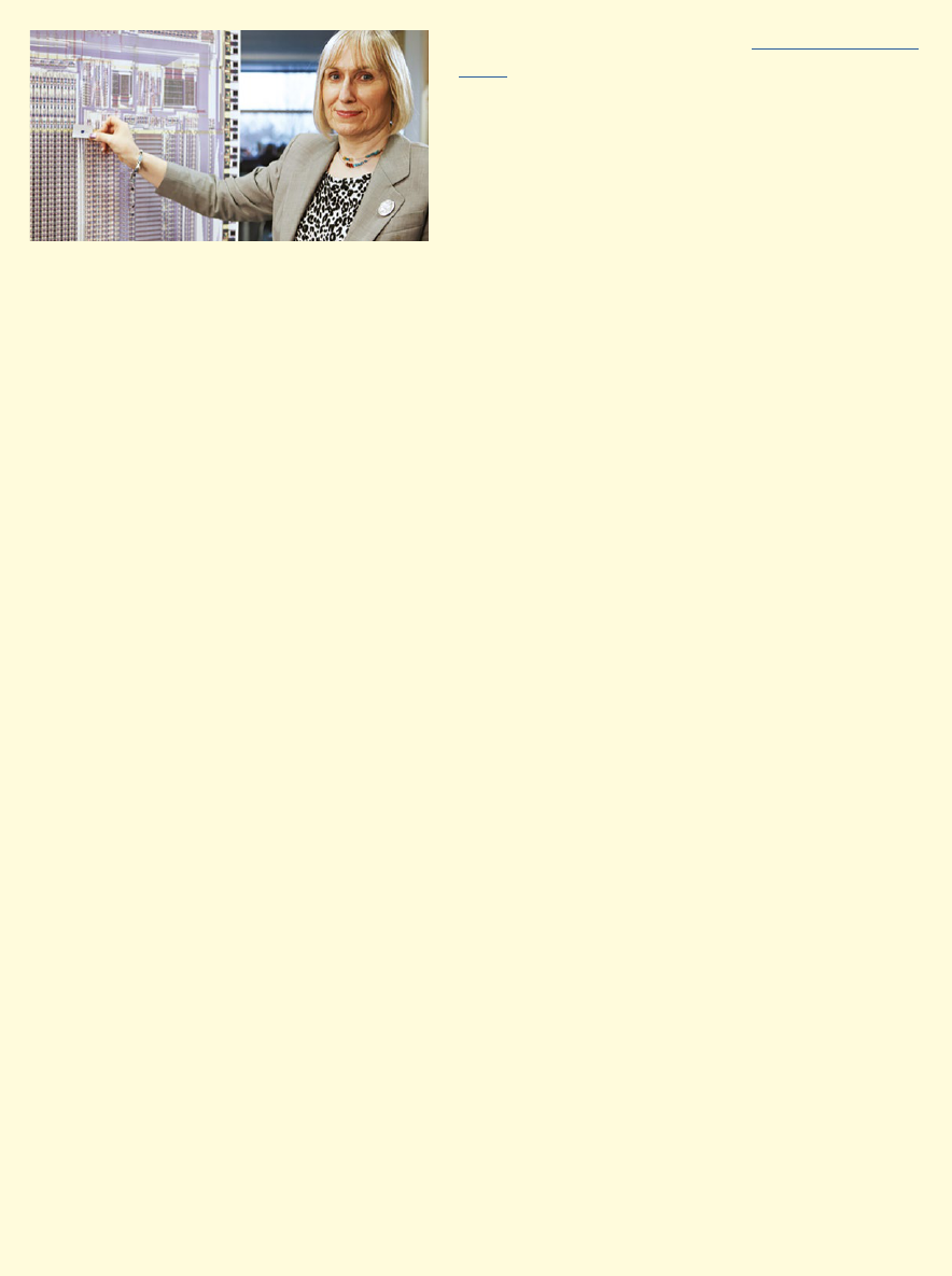
Operang Systems Foundaons with Linux on the Raspberry Pi
48
A brief history of Arm, based on an interview from
2012 with Sophie Wilson FRS FREng, a Brish
computer scienst and soware engineer who
designed the Acorn Micro-Computer and later
the instrucon set of the Arm processor, which
became the de facto model used in 21st-century
smartphones.
Image ©2013 Chris Monk, CC BY 2.0, commons.wikimedia.org
In 1983 Acorn Computers had produced the BBC Microcomputer. It was designed as a two-
processor system from the outset in order to be able to build both a small cheap machine and a big
expensive workstaon-style machine. This was possible by using two processors: an IO processor
and a second processor that would do the actual heavy liing. Acorn made many variants of the
second processor based on exisng microprocessors.
In Sophie’s words, "We could see what all these processors did and what they didn’t do. So, the rst
thing they didn’t do was they didn’t make good use of the memory system. The second thing they
didn’t do was that they weren’t fast, they weren’t easy to use." Regarding the raonale behind the
design of the original Arm processor, Sophie said, "We rather hoped that we could get to a power
level such that if you wrote in a higher-level language, you could , e.g., write 3D graphics games.
For the processors that were on sale at the me that wasn’t true. They were too slow. So we
felt we needed a beer processor. We parcularly felt we needed a beer processor in order to
compete with what was just beginning to be a ood of IBM PC compables. So, we gave ourselves
a project slogan which was MIPS for the masses". "This was very dierent to what other people were
doing at the me. RISC processor research had just been sort of released by IBM, by Berkeley, by
Stanford, and they were all aer making workstaon-class machines that were quite high end.
We ended up wanng to do the same thing but at the low end, a machine for the masses that
would be quite powerful but not super powerful."
"ARM was that machine: a machine that was MIPS for the masses. We started selling Arm powered
machines in 1986, 1987. The things that we’d endowed it with, what we’d set Arm up to be, with
its cheap and powerful mindset, were the things that became valuable. When people wanted to
put good amounts of processing into something, that was the really important aribute."
"We designed a deeply embedded processor, or an embedded processor, without consciously
realizing it in our striving for what we thought would be ideal for our marketplace; that’s been
what’s really maered. As a sort of side eect of making it cheap and simple to use, we also ended
up making it power ecient; that wasn’t intenonal. In hindsight, it was an obvious accident. We
only had 25,000 transistors in the rst one. We were worried about power dissipaon. We needed
to be extremely careful for something that would be mass manufactured and put into cheap
machines without heat sinks and that sort of thing. So there were already some aspects of power
conservaon in the design, but we performed way beer than that and as the world has gone
increasingly mobile that aspect of Arm has maered as well. But to start o, we designed a really
good, deeply embedded processor."
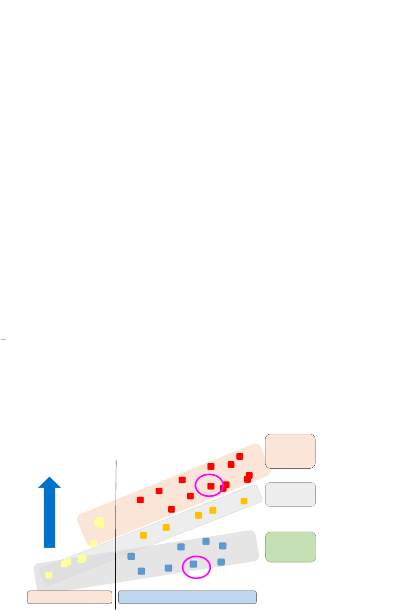
49
3.1 Overview
In this chapter, we discuss the hardware on which the operang system runs, with a focus on the
Linux view on the hardware system and the OS support of the Arm Cortex series processors. The
purpose of this chapter is to provide you with a useable mental model for the hardware system and
to explain the need for an operang system and how the hardware supports the OS.
What you will learn
Aer you have studied the material in this chapter, you will be able to:
1. Discuss the support that modern hardware oers for operang systems (dedicated registers, mers,
interrupt architecture, DMA).
2. Compare and contrast instrucon sets for the Arm Cortex M0+ and Arm Cortex A53 in terms of
purpose, capability and OS support.
3. Explain the role and structure of the address map.
4. Explain the hardware structure of the memory subsystem (caches, TLB, MMU).
3.2 Arm hardware architecture
Figure 3.1 [1] shows the enre Arm processor family, with the most recent members on the right, and
the highest performance and capability processors at the top. We will illustrate the Arm hardware
architecture using two quite dierent processors as examples: the Arm Cortex M0+ is a single-core,
very low gate count, highly energy-ecient processor that is intended for microcontroller and deeply
embedded applicaons that require an area opmized processor and low power consumpon, such as
IoT devices. It does not have a cache and uses the 16-bit Armv6-M Thumb instrucon set. In general,
such processors will not run Linux, however many of the main OS support features are sll available.
Figure 3.1: Arm processor family.
Application
Processors
(withMMU,
supportLinux,
MSmobileOS)
RealTime
Processors
Microcontrollers
anddeeply
embedded
Systemcapability&
perfo rmance
ARM7
TM
series
ARM920T
TM
,
ARM940T
TM
ARM946
TM
,
ARM966
TM
ARM926
TM
Cortex
-
M3
Cortex
-
M1
(FPGA)
Cortex
-
M0
Cortex
-
M0+
Cortex
-
M4
Cortex
-
R4
Cortex
-
R5
Cortex
-
R7
Cortex
-
A8
Cortex
-
A9
Cortex
-
A5
Cortex
-
A15
Cortex
-
A7
ARMCortexProcessors
ClassicARMProcessors
Cortex
-
A57
Cortex
-
A53
Cortex
-
A12
ARM11
T
M
series
Cortex
-
R8
Cortex
-
A17
Cortex
-
A72
Cortex
-
A73
Cortex
-
A32
Cortex
-
A35
Cortex
-
R52
Cortex
-
M7
Cortex
-
M23
Cortex
-
M33
Chapter 3 | Hardware architecture
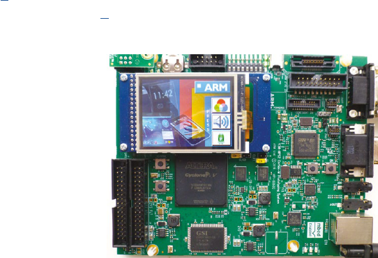
Operang Systems Foundaons with Linux on the Raspberry Pi
50
By contrast, the Arm Cortex A53, used in the Raspberry Pi 3, is a mid-range, low-power processor that
implements the Armv8-A architecture. The Cortex-A53 processor has one to four cores, each with an
L1 memory system and a single shared L2 cache. It is a 64-bit processor which supports the AArch64
and AArch32 (including Thumb) execuon modes. It is intended as an Applicaon Processor for
applicaon domains such as mobile compung, smartphones, and energy-ecient servers.
All Arm processor systems use the Advanced Microcontroller Bus Architecture (AMBA), an open-standard
specicaon for the connecon and management of funconal blocks in system-on-chip (SoC) designs.
All Arm processors have a RISC (Reduced Instrucon Set Compung) architecture
1
. RISC architecture
based processors typically require fewer transistors than those with a complex instrucon
set compung (CISC) architectures (e.g., x86), which can result in lower cost and lower power
consumpon. Furthermore, as the instrucons are simpler, most instrucons can be executed in a
single cycle, which makes instrucon pipelining simpler and more ecient. The complex funconality
supported in a CISC instrucon set is achieved through a combinaon of mulple RISC instrucons.
Typically, RISC machines have a large number of general-purpose registers (while CISC machines
have more special-purpose registers). In a RISC architecture, any register can contain either data or an
address. Furthermore, a RISC processor typically operates on data held in registers. Separate load and
store instrucons transfer data between the register bank and external memory (this is called a load-
store architecture).
3.3 Arm Cortex M0+
The Arm Cortex-M0+ processor is a low-spec embedded processor, typically used for applicaons
that need lower power and don’t need full OS support. Figure 3.2 shows the Arm MPS2+ Prototyping
Board for Cortex-M based designs, an FPGA development plaorm supporng the enre Cortex-M
processor range except for the M23 and M33. The funconal block diagram of the Cortex-M0+
processor [2] is shown in Figure 3.3. The Cortex-M0+ uses the AHB-Lite (Advanced High-performance
Bus Lite) Lite bus standard [3]. AHB-Lite is a bus interface that supports a single bus master and
provides high-bandwidth operaon.
Figure 3.2: Arm MPS2+ FPGA Prototyping Board for Cortex-M based designs. Photo by author.
1
The name ARM was originally an acronym for Acorn RISC Machine and was altered to Advanced RISC Machines.
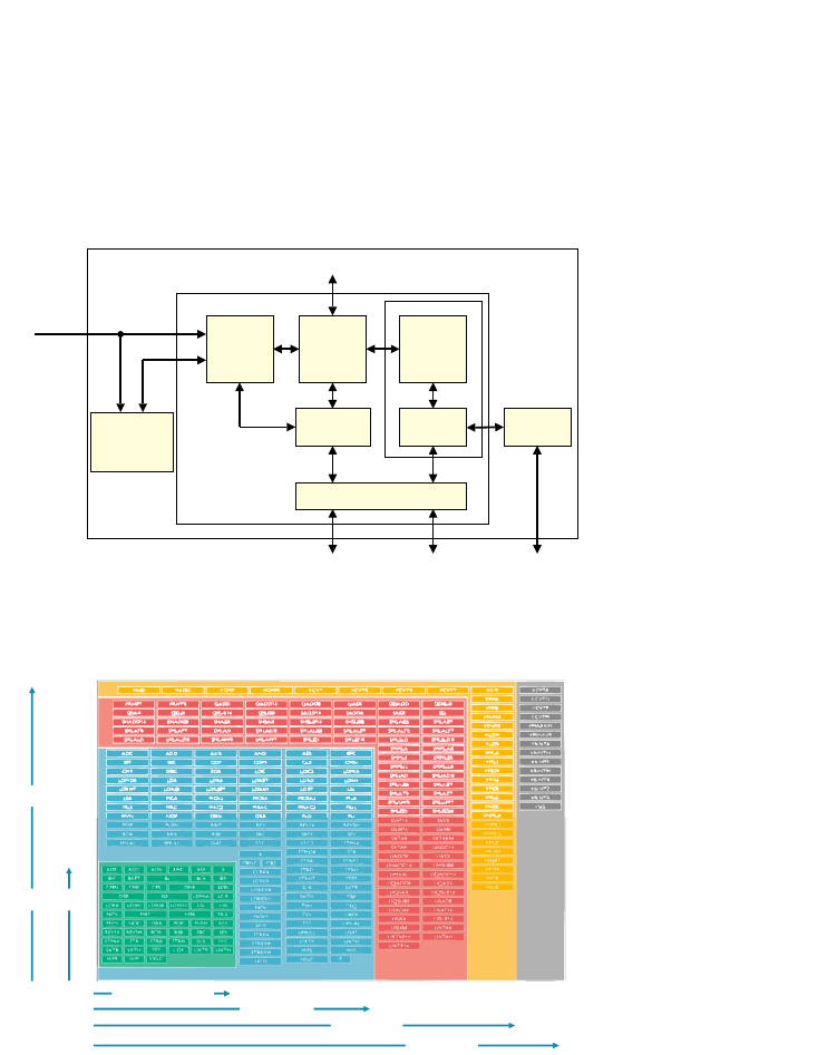
51
It is typically used to communicate with internal memory devices, external memory interfaces, and
high bandwidth peripherals. Low-bandwidth peripherals can be included as AHB-Lite slaves but
typically reside on the AMBA Advanced Peripheral Bus (APB). Bridging between AHB and APB is done
using a AHB-Lite slave, known as an APB bridge.
Figure 3.3: Cortex-M0 processor funconal block diagram.
Figure 3.4: Thumb instrucon set support in the Cortex-M processors.
3.3.1 Interrupt control
The Cortex-M0+ handles interrupts via a programmable controller called the Nested Vectored
Interrupt Controller (NVIC). This controller supports up to 240 dynamically re-priorizable interrupts
each with up to 256 levels of priority. It keeps track of stacked/nested interrupts to enable back-to-
back processing (“tail-chaining”) of interrupts.
3.3.2 Instrucon set
As menoned, the Cortex-M0+ implements the Armv6-M Thumb instrucon set; this is a subset
of the Armv7-M Thumb instrucon set and includes a number of 32-bit instrucons that use
Thumb-2 technology. The Thumb instrucon set is a 16-bit instrucon set formed of a subset of the
Cortex-M0+ processor
Cortex-M0+
processor
core
Bus matrix
Nested
Vectored
Interrupt
Controller
(NVIC)
Interrupts
‡Wakeup
Interrupt
Controller (WIC)
‡Debug
Access Port
(DAP)
AHB-Lite interface
to system
‡Serial Wire or
JTAG debug port
‡ Optional component
Debug
‡Debugger
interface
‡Breakpoint
and
watchpoint
unit
Cortex-M0+ components
‡Memory
protection unit
Execution Trace Interface
‡Single-cycle
I/O port
Cortex-M0/M0+
Cortex-M3
Cortex-M4
Cortex-M7
ARMv6-M
ARMv7-M
Advanced data processing
bit field manipulations
General data processing
I/O control tasks
DSP (SIMD, fast MAC)
Floating Point
Chapter 3 | Hardware architecture

Operang Systems Foundaons with Linux on the Raspberry Pi
52
most commonly used 32-bit Arm instrucons. Thumb instrucons have corresponding 32-bit Arm
instrucons that have the same eect on the processor model. Thumb instrucons operate with
the standard Arm register conguraon. On execuon, 16-bit Thumb instrucons are transparently
decompressed to full 32-bit Arm instrucons in real-me, without performance loss. For more details,
we refer to [2]. Figure 3.4 illustrates the various Arm Thumb instrucon sets and the purposes of the
instrucons. The key points to noce is that the Armv6-M Thumb instrucon set is very small and that
it is a very reduced subset of the complete Thumb instrucon set.
3.3.3 System mer
An interesng feature of the Cortex-M0+ is the oponal 24-bit System Timer (SysTick). This mer
can be used by an operang system. It can be polled by soware or can be congured to generate an
interrupt. The SysTick interrupt has its own entry in the vector table and therefore can have its own
handler. The SysTick mer is controlled via a set of special system control registers.
3.3.4 Processor mode and privileges
The Cortex-M0+ processor supports the Armv6-M Thread and Handler mode through a control
register (CONTROL) and two dierent stack pointers, Main Stack Pointer (MSP) and Process Stack
Pointer (PSP) as explained in Chapter 1. Thread mode is used to execute applicaon soware. The
processor enters Thread mode when it comes out of reset. Handler mode is used to handle excepons.
The processor returns to Thread mode when it has nished all excepon processing.
It also (oponally) supports dierent privilege levels for soware execuon as follows:
Unprivileged: The soware has limited access to the MSR and MRS instrucons, and cannot use the
CPS instrucon or access the system mer, NVIC, or system control block. It might have restricted
access to memory or peripherals.
Privileged: The soware can use all the instrucons and has access to all resources.
In Thread mode, the CONTROL register controls whether soware execuon is privileged or
unprivileged. In Handler mode, soware execuon is always privileged. Only privileged soware can
write to the CONTROL register to change the privilege level for soware execuon in Thread mode.
Unprivileged soware can use the SVC instrucon to make a supervisor call to transfer control to
privileged soware.
3.3.5 Memory protecon
The Cortex-M0+ (oponally) supports memory protecon through an oponal Memory Protecon
Unit (MPU). When implemented, the processor supports the Armv6 Protected Memory System
Architecture model [2]. The MPU provides support for protecon regions with priories and access
permissions. The MPU can be used to enforce privilege rules, separate processes, and manage
memory aributes.
Considering the above features, in principle, the M0+ is capable of running an OS like Linux. In
pracce, embedded systems with a Cortex-M0+ will not have sucient storage and memory to run
Linux, but they can support other OSs such as freeRTOS.
2
2
hps://www.freertos.org/
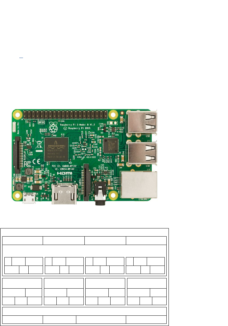
53
3.4 Arm Cortex A53
This processor is used in the Raspberry Pi 3, shown in Figure 3.5. The funconal block diagram of
the Cortex-A53 processor [4] is shown in Figure 3.6. It is immediately clear that this is a much more
complex processor, with up to 4 cores and a 2-level cache hierarchy. Each core (boom row) has a
dedicated Floang-point Unit (FPU) and the Neon SIMD (single instrucon mulple data) architecture
extension. From the Governor blocks at the top, the main features of interest from an OS perspecve
are “Arch mer” and “GIC CPU interface.” The other blocks (CTI, Retenon control, and Debug over
power down) provide advanced debug and power-saving support.
Figure 3.5: Raspberry Pi 3 Model B with Arm Cortex-A53. Photo by author.
Figure 3.6: Cortex-A53 processor funconal block diagram.
3.4.1 Interrupt control
The “GIC CPU interface” block represents the Generic Interrupt Controller CPU Interface, an
implementaon of the Generic Interrupt Controller (GIC) architecture dened as part of the Armv8-A
architecture. The GIC denes the architectural requirements for handling all interrupt sources
for any processing element connected to a GIC and a common interrupt controller programming
L1
ICache
L1
DCache
Debug
and trace
Core 0
L2 cache SCU
ACE/AMBA 5 CHI
master bus interface
ACP slave
Level 2 memory system
Core 0 governor
L1
ICache
L1
DCache
Debug
and trace
Core 1
FPU and NEON
extension
Crypto
extension
L1
ICache
L1
DCache
Debug
and trace
Core 2
L1
ICache
L1
DCache
Debug
and trace
Core 3
Core 1 governor Core 2 governor Core 3 governor
Arch
timer
GIC CPU
interface
Clock and
reset
CTI
Retention
control
Debug over
power down
Arch
timer
GIC CPU
interface
Clock and
reset
CTI
Retention
control
Debug over
power down
Arch
timer
GIC CPU
interface
Clock and
reset
CTI
Retention
control
Debug over
power down
Arch
timer
GIC CPU
interface
Clock and
reset
CTI
Retention
control
Debug over
power down
Governor
APB decoder APB ROM APB multiplexer CTM
Cortex-A53 processor
FPU and NEON
extension
Crypto
extension
FPU and NEON
extension
Crypto
extension
FPU and NEON
extension
Crypto
extension
Chapter 3 | Hardware architecture
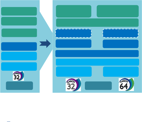
Operang Systems Foundaons with Linux on the Raspberry Pi
54
interface applicable to uniprocessor or mulprocessor systems. The GIC is a much more advanced
and exible interrupt handling system than the NVIC of the Cortex-M0+ because it needs to support
heterogeneous mulcore systems and virtualizaon. Rather than the simple set of registers used by
the NVIC, the GIC uses a memory-mapped interface of 255KB as well as a set of GIC control registers
(GICC*) and registers to support virtualizaon of interrupts (GICH*, GICV*) in the CPU.
3.4.2 Instrucon set
The Cortex-A53 supports both the AArch32 and AArch64 instrucon set architectures. The AArch32
includes the Thumb instrucon set used in the Cortex-M series. Consequently, code compiled for
the Cortex-M0+, for example, can run on the Cortex-A53. More to the point, the Raspbian Linux
distribuon for the Raspberry Pi 3 is a 32-bit distribuon, so the processor is running the OS and all
applicaons in the AArch32 state.
Figure 3.7: Arm architecture evoluon.
Figure 3.7, adapted from [5], shows how the Armv7-A architecture has been incorporated into the
Armv8-A architecture. In addion, Armv8 supports two execuon states: AArch32, in which the A32
and T32 instrucon sets (Arm and Thumb in Armv7-A) are supported and AArch64, in the 64-bit
instrucon set. Armv8-A is backwards compable with Armv7-A, but the excepon, privilege, and
security model has been signicantly extended as discussed below. In AArch32, the Armv7-A Large
Physical Address Extensions are supported, providing 32-bit virtual addressing and 40-bit physical
addressing. In AArch64, this is extended in a backward compable way to provide 64-bit virtual
addresses and a 48-bit physical address space. Another addion is the cryptographic at the instrucon
level, i.e., dedicated instrucons to speed up cryptographic computaons.
The latest ISO/IEC standards for C (C11, ISO/IEC 9899:2011) and C++ (ISO/IEC 14882:2011)
introduce standard capabilies for mul-threaded programming. This includes the requirement for
standard implementaons of mutexes and other forms of "uninterrupble object access." The Load-
Acquire and Store-Release instrucons introduced in AArch64 have been added to comply with these
standards.
LargePhysAddrExtn
VirtualizationExtn
TrustZone
ARM+Thumb ISAs
NEON
Hard_Float
ARMv7-A
ARMv8-A
AdvSIMD
( SP float)
AdvSIMD
( SP+DP float)
IEEE 754-2008 compliant floating point
LD acquire/ST release: C1x/C++11 compliance
A32+T32 ISAs
A64 ISA
Crypto
EL3, EL2, EL1 and EL0 exception hierarchy
{4, 16, 64}KB pages
4KB pages
32-bit VA;≤40-bit PA
>32-bit VA;≤48-bit PA
32
32
Crypto

55
Floang-point and SIMD support
The Armv8 architecture provides support for IEEE 754-2008 oang-point operaons and SIMD
(Single Instrucon Mulple Data) or vector operaons through dedicated registers and instrucons.
The Armv8 architecture provides two register les, a general-purpose register le, and a SIMD and
oang-point register (SIMD&FP) register le. In each of these, the possible register widths depend on
the Execuon state.
In AArch64 state, there is:
A general-purpose register le containing 31 64-bit registers. Many instrucons can access these
registers as 64-bit registers or as 32-bit registers, using only the boom 32 bits.
A SIMD&FP register le containing 32 128-bit registers. The quadword integer and oang-point
data types only apply to the SIMD&FP register le. The AArch64 vector registers support 128-
bit vectors (the eecve vector length can be 64-bits or 128-bits depending on the instrucon
encoding used).
In AArch32 state, there is:
A general-purpose register le containing 32-bit registers. Two 32-bit registers can support
a doubleword; vector formang is supported.
A SIMD&FP register le containing 64-bit registers. AArch32 state does not support quadword
integer or oang-point data types.
Both AArch32 and AArch64 states support SIMD and oang-point instrucons:
AArch32 state provides:
SIMD instrucons in the base instrucon sets that operate on the 32-bit general-purpose
registers.
Advanced SIMD instrucons that operate on registers in the SIMD&FP register le.
Floang-point instrucons that operate on registers in the SIMD&FP register le.
AArch64 state provides:
Advanced SIMD instrucons that operate on registers in the SIMD&FP register le.
Floang-point instrucons that operate on registers in the SIMD&FP register le.
Chapter 3 | Hardware architecture

Operang Systems Foundaons with Linux on the Raspberry Pi
56
3.4.3 System mer
The Arm Cortex-A53 implements the Arm Generic Timer architecture [6]. The Generic Timer can
schedule events and trigger interrupts based on an incremenng counter value. It provides:
Generaon of mer events as interrupt outputs.
Generaon of event streams.
The Generic Timer can schedule events and trigger interrupts based on an incremenng counter value.
It provides a system counter that measures the passing of me in real-me but also supports virtual
counters that measure the passing of virtual-me, i.e., the “equivalent real-me” on a Virtual Machine.
The Cortex-A53 processor provides a set of mer registers within each core of the cluster. The mers are:
An EL1 Non-secure physical mer.
An EL1 Secure physical mer.
An EL2 physical mer.
A virtual mer.
The Cortex-A53 processor does not include the system counter. This resides in the SoC. The system
counter value is distributed to the Cortex-A53 processor with a synchronous binary encoded 64-bit
bus. For more details, we refer to the Technical Reference Manual [4].
3.4.4 Processor mode and privileges
In terms of privileges, the Cortex-A53 denes the Armv8 excepon model, with four Excepon levels,
EL0-EL3, that provide an execuon privilege hierarchy:
EL0 has the lowest soware execuon privilege, and execuon at EL0 is called unprivileged
execuon.
Increased values of n, from 1 to 3, indicate increased soware execuon privilege. The OS would
run in EL1.
EL2 provides support for processor virtualizaon.
EL3 provides support for two security states, as part of the TrustZone architecture:
In Secure state, the processor can access both the Secure and the Non-secure memory address
space. When execung at EL3, it can access all the system control resources.
In Non-secure state, the processor can access only the Non-secure memory address space and
cannot access the Secure system control resources.

57
The addion of EL3 allows, e.g. to run a trusted OS in parallel with a hypervisor supporng non-
trusted OSs on a single system.
It is possible to switch at run me between the AArch32 and AArch64 instrucon set architectures,
but there are certain restricons relang to the excepon levels, explained in Figure 3.8. Essenally,
code running at a higher excepon level can only be AArch64 if the lower excepon levels are also
AArch64.
Figure 3.8: Moving between AArch32 and AArch64.
For each implemented Excepon level, in AArch64 state, a dedicated stack pointer register is
implemented. In AArch32 state, the stack pointer depends on the “PE mode” (these do not exist in
AArch64). PE modes support normal soware execuon and handle excepons. The current mode
determines the set of general-purpose and special-purpose registers that are available. The AArch32
modes are:
Monitor mode. This mode always executes at Secure EL3.
Hyp (hypervisor) mode. This mode always executes at Non-secure EL2.
System, Supervisor, Abort, Undened, IRQ, and FIQ modes. The Excepon level these modes
execute at depends on the Security state:
In Secure state: Execute at EL3 when EL3 is using AArch32.
In Non-secure state: always execute at EL1.
User mode. This mode always executes at EL0.
3.4.5 Memory management unit
As explained in Chapter 1, modern processors provide hardware support for address translaon and
memory protecon. We also explained briey the concept of memory pages and the page table.
A more detailed discussion is provided in Chapter 6, “Memory management.” For the purpose of the
discussion of the Cortex-A53 MMU, we can consider the terms “virtual memory” and “logical memory”
to be the same. An addional complexity is caused by the support for Virtual Machines (hypervisor) in
AArch64
App
EL0
EL1
EL2
An AArch64
OS can host
a mix of
AArch64
and AArch32
applications
An AArch32
OS cannot host
an AArch64
application
An AArch32
hypervisor
cannot host
an AArch64 OS
An AArch64
hypervisor
can host
an AArch64 and
AArch32 OS
AArch64 OS AArch32 OS
Hypervisor
AArch32
App
AArch32
App
AArch64
App
Chapter 3 | Hardware architecture
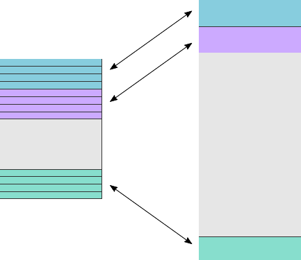
Operang Systems Foundaons with Linux on the Raspberry Pi
58
the Armv8 architecture: as each VM must provide the illusion of running on real hardware, there is an
extra level of addressing called Intermediate Physical Address (IPA) required.
The MMU controls table walk hardware that accesses translaon tables in main memory. It translates
virtual addresses to physical addresses and provides ne-grained memory system control through
a set of virtual-to-physical address mappings and memory aributes held in page tables.
These are loaded into the Translaon look-aside buer (TLB) when a locaon is accessed. In pracce,
the TLB is split into a very small, very fast micro TLB and a larger main TLB.
The MMU in each core comprises the following components:
Translaon look-aside buer
The TLB consists of two levels:
1. A 10-entry fully-associave instrucon micro TLB and 10-entry fully-associave data micro TLB.
We explained the concept of a fully-associave cache in Chapter 1. There are two separate micro
TLBs for instrucons and data to allow parallel access for performance reasons.
2. A 4-way set-associave 512-entry unied main TLB (Figure 3.9). “Unied” means that this TLB is
used for both instrucons and data. The main TLB is not fully associave but 4-way set-associave.
Remember that “fully associave” means that every address can be stored at any possible entry of the
TLB. If the cache or TLB is not fully associave, it means that there are restricons on where a given
address can be stored. A very common approach is an n-way set-associave cache, which means that
the cache is divided into blocks of n entries, and each block is mapped to a xed region of memory.
An address from a given region of memory can only be stored in a given block, but it can be stored in
any of the n entries in that block. For example, on the Raspberry Pi 3, the RAM is 1GB. Given a page
size of 4kB, this means 256K pages. This is mapped to 128 blocks (4 entries per block in the TLB), so
every physical memory block has 2k frames, each of which can be stored in one of 4 entries in the TLB.
Figure 3.9: 4-way set-associave main TLB.
Set 1
entry 1
entry 2
entry 3
entry 4
Set 2
Set 128
entry 1
entry 2
entry 3
entry 4
entry 1
entry 2
entry 3
entry 4
Block 1
Block 1
Block 128
512-entry TLB
1GB memory,
page size 4kB
2,048 frames
per block
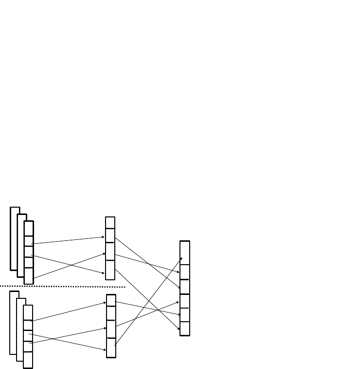
59
Addional caches
As we will see in Chapter 6, in pracce page tables are hierarchical and address translaon in a hypervisor-
based environment has two stages (Figure 3.10). The Cortex-53 MMU, therefore, provides addional caches:
4-way set-associave 64-entry walk cache.
The walk cache RAM holds the paral result of a stage 1 translaon. For more details, see Chapter 6.
4-way set-associave 64-entry IPA cache.
The Intermediate Physical Address (IPA) cache RAM holds mappings between intermediate physical
addresses and physical addresses. Only Non-secure EL1 and EL0 stage 2 translaons use this cache.
Note that it is possible to disable stage 1 or stage 2 of the address translaon.
Figure 3.10: Two-stage address translaon.
3.4.6 Memory system
In Chapter 1, we introduced the concept of caching and a simple model for a cache, a small, fast
memory for oen-used data. The actual memory system in the Cortex-A53 is more complicated, but
the same concepts apply (Figure 3.6).
L1 Cache
The L1 memory system consists of separate per-core instrucon and data caches. The implementer
congures the instrucon and data caches independently during implementaon, to sizes of 8KB,
16KB, 32KB, or 64KB. The Raspberry Pi 3 conguraon has 16KB for both Instrucon and Data.
Note that the instrucon cache is read-only because instrucon memory is read-only.
The L1 instrucon cache has the following key features:
Cache line size of 64 bytes.
2-way set associave.
“Physical” address (≤40-bit IPA)
map of each Guest OS
Translation
performed by
the
Hypervisor
Physical address
(≤40
-bit PA) map
Virtual address (32-bit VA) map of
each application on each Guest OS
Translations by
each Guest OS
Translations by
each Guest OS
Chapter 3 | Hardware architecture
Operang Systems Foundaons with Linux on the Raspberry Pi
60
16-byte read interface to the L2 memory system. This means it takes 4 cycles to read a cache line
from the L2 cache.
The L1 data memory system has the following features:
Cache line size of 64 bytes.
4-way set associave.
32-byte write and 16-byte read interface to the L2 memory system.
64-bit read and 128-bit write path from the data L1 memory system to the datapath. In other
words, the CPU can read one 64-bit word and write 2 64-bit words directly from the L1 data cache.
Support for three outstanding data cache misses. This means that instead of immediately fetching
a cache line on a cache miss, the requests are deferred. So the cache will not block to fetch the
cache line on the rst miss but allow the CPU to connue execung instrucons (and hence
potenally create more misses).
The L1 data cache supports only a Write-Back policy (remember from Chapter 1, this means that
inial writes are to the cache, and write back to memory only occurs on evicon of the cache line).
It normally
3
allocates a cache line on either a read miss or a write miss (i.e., both write-allocate and
read-allocate). A special feature of the L1 data cache is that it includes logic to switch into pure read
allocate mode for certain scenarios. When in read allocate mode, loads behave as normal, and writes
sll lookup in the cache but, if they miss, they write out to L2 only.
The L1 data cache uses physical memory addresses. The micro TLB produces the physical address
from the virtual address before performing the cache access.
L2 Cache
The L2 cache is a unied cache shared by all cores, with a congurable cache size of 128KB, 256KB,
512KB, 1MB, and 2MB. The Raspberry Pi 3 conguraon is 512KB.
Data is allocated to the L2 cache only when evicted from the L1 memory system, not when rst
fetched from the system. Instrucons are allocated to the L2 cache when fetched from the system
and can be invalidated during maintenance operaons.
The L2 cache has the following key features:
Cache line size of 64 bytes;
16-way set-associave cache structure;
Uses physical addresses.
3
This behavior can be altered by changing the inner cache allocaon hints in the page tables.
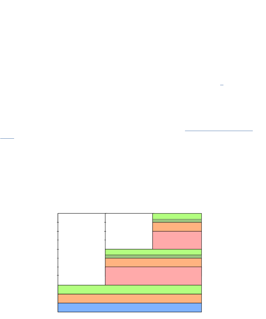
61
Data cache coherency
Cache coherency refers to the need to ensure that local caches on dierent cores in a mulcore
system with a shared memory have present a coherent view on the memory. This essenally
means that the system should behave as if there are no caches. We note for completeness that the
Cortex-A53 processor uses the MOESI protocol to maintain data coherency between mulple cores.
In this protocol, each cache line is in one of ve states: Modied, Owned, Exclusive, Shared, or Invalid.
The L2 memory system includes a Snoop Control Unit (SCU) which implements this protocol. For more
informaon, we refer to the "Arm Cortex-A Series Programmer’s Guide for ARMv8-A", [7].
3.5 Address map
The descripon of the purpose, size, and posion of the address regions for memory and peripherals
in a system is called the address map or memory map. Because Arm system can be 32 or 64-bit, the
address space ranges from 4GB (32-bit) to 1TB (40-bit). The white paper Principles of Arm Memory
Maps describes Arm address maps for 32, 36 and 40-bit systems, and proposes extensions for 44 and
48-bit systems.
Arm has harmonized the memory maps across its various systems to provide internal consistency and
soware portability, and to address the constraints that come with mixing 32-bit components within
larger address spaces. The introducon of Large Physical Address Extension (LPAE) to ARMv7 class
CPUs has grown the physical address spaces to 36-bit and 40-bits, providing 64GB or 1024GB (1TB)
memory space. The 64-bit ARMv8 architecture can address 48-bits, providing 256TB.
Figure 3.11: Arm 40-bit address map.
Figure 3.11 shows how the address maps for dierent bit widths are related. The address maps are
dened as nested sets. As each memory map increases by 4-bits of address space, it contains all of
0 GB
1 GB
2 GB
4 GB
8 GB
16 GB
32 GB
64 GB
128 GB
256 GB
512 GB
1024 GB
32-bit
36-bit
40-bit
Mapped I/O
DRAM
Reserved
Mapped I/O
DRAM
Reserved
Mapped I/O
2 GB of DRAM
ROM & RAM & I/O
32-bit 36-bit 40-bit
0
32-bit
36-bit
40-bit
32 GB hole or DRAM
2 GB hole or DRAM
Log2 scale
Chapter 3 | Hardware architecture
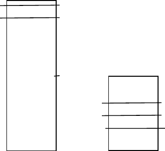
Operang Systems Foundaons with Linux on the Raspberry Pi
62
the smaller address maps, at the lower addresses. Each increment of 4 address bits results in a 16-fold
increase in addressable space. The address space is paroned in a repeatable way:
8/16 DRAM;
4/16 Mapped I/O;
3/16 Reserved space;
1/16 Previous memory map (i.e., without the addional 4 address bits).
For example, the 36-bit address map contains the enre 32-bit address map in the lowest 4GB of
address space.
The address maps are paroned into four types or regions:
1. Stac I/O and Stac Memories, for register, mapped on-chip peripherals, boot ROMs,
and scratch RAMs.
2. Mapped I/O, for dynamically congured, memory-mapped buses, such as PCIe.
3. DRAM, for main system dynamic memory.
4. Reserved space, for future use.
The “DRAM holes” menoned in the Figure are an oponal mechanism to simplify the decoding
scheme when paroning a large capacity DRAM device across the lower physically addressed
regions, at the cost of leaving a small percentage of the address space unused.
Figure 3.12: Broadcom BCM2835 Arm-based SoC (Raspberry Pi) address maps.
I/O Peripherals
0x80000000
(2GB)
0x7E000000
(start of 32MB range)
0x40000000
(1GB)
00000000
I/O Peripherals
0x20000000
(I/O base set
in arm loader)
System
SDRAM
CPU bus
addresses
Arm physical
addresses
0x40000000
(1GB)
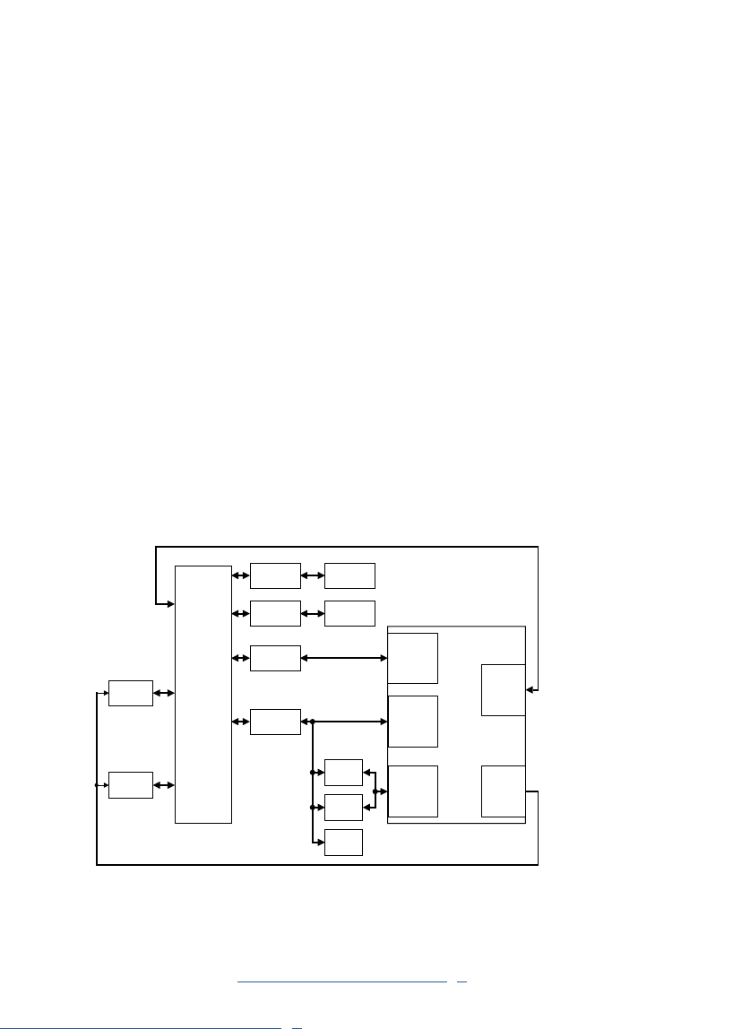
63
If we consider the 32-bit address space in the case of the Broadcom BCM2835 System-on-Chip used
in the Raspberry Pi 3, the picture (Figure 3.12 ) is a bit more complicated because the actual 32-bit
address space is used for the addresses on the system bus, but an MMU translates these addresses
to a dierent set of “physical” addresses for the Arm CPU. The lowest 1GB of the Arm physical
address map is eecvely the Linux kernel memory. For addressing of user memory, an addional
MMU is used.
3.6 Direct memory access
Direct memory access (DMA) is a mechanism that allows blocks of data to be transferred to or from
devices with no CPU overhead. The CPU manages DMA operaons by subming DMA requests to
a DMA controller. While the DMA transfer is in progress, the CPU can connue execung code. When
the DMA transfer is completed, the DMA controller signals the CPU via an interrupt.
DMA is advantageous if large blocks of memory have to be copied or if the transfer is repeve
because both cases would otherwise consume a considerable amount of CPU me. Like most modern
operang systems, Linux supports DMA transfers through a kernel API, if the hardware has DMA
support. It should be noted that this does not require special instrucons:the DMA controller is
memory-mapped, and the CPU simply writes the request to that region of memory.
Figure 3.13: Example system with Cortex-A and CoreLink DMA controller.
Arm processors do not include a DMA engine as part of the CPU core. Arm provides dedicated
DMA controllers such as the lightweight PrimeCell µDMAController [8], a very low gate count DMA
controller compable with the AMBA AHB-Lite protocol as used in the Cortex-M series, and the more
advanced CoreLink DMA-330 DMA Controller [9] which has a full AMBA-compliant interface or the
SoC manufacturers can provide their own DMA engines. Figure 3.13 shows an example system with
the CoreLink DMAC. In the Arm Cortex M series, the DMA controller will be a peripheral on the
AHB bus.
SMC
DMC DRAM
Flash
memory
Secure
APB slave
interface
AXI
master
interface
DMAC
AXI
Interconnect
AXI-APB
bridge
GPIO
Non-
secure
APB slave
interface
Peripheral
request
interface
Interrupt
outputs
AXI-APB
bridge
UART
Timer
ARM
processor
ARM
processor
Chapter 3 | Hardware architecture

Operang Systems Foundaons with Linux on the Raspberry Pi
64
However, in the higher-end Arm Cortex-A series, a special interface called Accelerator Coherency Port
(ACP) is provided as part of the AMBA AXI standard. The reason is that on mulcore processors with
cache coherency, the cache system complicates the DMA transfer because it is possible that some
data has not been wrien to the main memory at the me of the transfer. With the ACP, the Cortex-A
series implement a hardware mechanism to ensure that accesses to shared DMA memory regions are
cache-coherent. Without such a mechanism, the operang system (or end-user soware on a bare-
metal system) must ensure the coherency. More details on integrang a DMA engine in an Arm-based
mulprocessor SoC are provided in the Applicaon Note Implemenng DMA on ARM SMP Systems [10].
On the Arm Cortex A53, the ACP port is oponal, and it is not provided on the SoC in the Raspberry
Pi 3. The DMA controller on the Raspberry Pi SoC is not a ARM IP core. It is part of the I/O Peripheral
address space. An addional complicaon, in this case, is that the DMA controller uses CPU bus
addresses so for a DMA transfer the soware needs to translate between the Arm physical addresses
and the CPU bus addresses.
In general, DMA controllers are complex devices that usually have their own instrucon set as well as
a register le. This means that the Linux kernel needs a dedicated driver for the DMA controller.
3.7 Summary
In this chapter, we had a look a two dierent types of Arm processors: the Arm Cortex M0+, a single-
core, very low gate count, highly energy-ecient processor intended for microcontroller and deeply
embedded applicaons that implements the ARMv6-M architecture, and the Arm Cortex A53 used in
the Raspberry Pi 3, a mid-range, low-power processor that implements the Armv8-A architecture and
has all features required to run an OS like Linux. We have discussed these processors in terms of their
instrucon set, interrupt model, security model, and memory system. We have also introduced the
Arm address maps and Direct memory access (DMA) support.
3.8 Exercises and quesons
3.8.1 Bare-bones programming
The aim of this exercise is to implement some of the basic operang system funconality. To do this
from scratch is quite a lot of work but we suggest you start from exisng code provided in the tutorial
series Bare-Metal Programming on Raspberry Pi 3 on GitHub.
1. Create a cyclic execuve with three tasks where each task creates a connuous waveform: task 1
creates a sine; task 2, a block wave; and task 3, a triangle; each with a dierent period. Print either
the values of the waveforms or a text-based graph on the terminal.
2. Make your cyclic execuve preempve.
3. Share a resource between the three tasks. This can be a simple shared variable with read and write
access.

65
Other, harder suggesons:
1. Make memory allocaon dynamic, i.e., write your own malloc() and free().
2. Create a minimal memory le system.
3.8.2 Arm hardware architecture
1. What was the meaning of “MIPS for the masses”?
2. What are the advantages of a RISC architecture over a CISC architecture?
3.8.3 Arm Cortex M0+
1. For what kind of projects would you use an Arm Cortex M0+?
2. Why is the Arm Cortex M0+ not suitable for running Linux?
3.8.4 Arm Cortex A53
1. Discuss oang-point and SIMD support in the Arm Cortex A53
2. Discuss the processor modes and privileges in the Arm Cortex A53
3. Discuss the cache and TLB architecture of the Arm Cortex A53
3.8.5 Address map
1. Explain why Arm systems share a common address map for 32, 36 and 40-bit systems.
2. What is the purpose of “DRAM holes”?
3.8.6 Direct memory access
1. What is the role of the Accelerator Coherency Port (ACP) in the DMA architecture?
Chapter 3 | Hardware architecture

Operang Systems Foundaons with Linux on the Raspberry Pi
66
References
[1] J. Yiu, Arm Cortex-M for Beginners – An overview of the Arm Cortex-M processor family and comparison, Arm Ltd, 3 2017, v2. [Online].
Available: hps://developer.arm.com/-/media/Files/pdf/Porng%20to%20ARM%2064-bit%20v4.pdf
[2] Cortex™-M0+ Technical Reference Manual Revision: r0p1, Arm Ltd, 12 2012, revC. [Online].
Available: hp://infocenter.arm.com/help/topic/com.arm.doc.ddi0484c/DDI0484C_cortex_m0p_r0p1_trm.pdf
[3] AMBA 3 AHB-Lite Protocol – Specicaon, Arm Ltd, 3 2017, v1.0. [Online].
Available: hps://silver.arm.com/download/download.tm?pv=1085658
[4] Arm
®
Cortex
®
-A53 MPCore Processor – Technical Reference Manual Rev: r0p4, Arm Ltd, 2 2016, revision: r0p4. [Online].
Available: hp://infocenter.arm.com/help/topic/com.arm.doc.ddi0500g/DDI0500G_cortex_a53_trm.pdf
[5] C. Shore, Porng to 64-bit Arm, Arm Ltd, 7 2014, revC. [Online].
Available: hps://developer.arm.com/-/media/Files/pdf/Porng%20to%20ARM%2064-bit%20v4.pdf
[6] ARM
®
Architecture Reference Manual – ARMv8, for ARMv8-A architecture prole, Arm Ltd, 12 2017, issue: C.a. [Online].
Available: hps://silver.arm.com/download/download.tm?pv=4239650&p=1343131
[7] Arm Cortex-A Series - Programmer’s Guide for ARMv8-A - Version: 1.0, Arm Ltd, 3 2015, issue A. [Online].
Available: hp://infocenter.arm.com/help/topic/com.arm.doc.den0024a/DEN0024A_v8_architecture_PG.pdf
[8] PrimeCell uDMA Controller (PL230) Technical Reference Manual Revision: r0p0, Arm Ltd, 1 2007, issue: A. [Online].
Available: hp://infocenter.arm.com/help/index.jsp?topic=/com.arm.doc.ddi0417a/index.html
[9] CoreLink DMA-330 DMA Controller Technical Reference Manual Revision: r1p2, Arm Ltd, 1 2012, issue: D. [Online].
Available: hp://infocenter.arm.com/help/index.jsp?topic=/com.arm.doc.ddi0424d/index.html
[10] Implemenng DMA on ARM SMP Systems, Arm Ltd, 8 2009, issue: A. [Online].
Available: hp://infocenter.arm.com/help/index.jsp?topic=/com.arm.doc.dai0228a/index.html

67
Chapter 3 | Hardware architecture

Chapter 4
Process management

Operang Systems Foundaons with Linux on the Raspberry Pi
70
4.1 Overview
Processes are programs in execuon. Have you ever seen a whale skeleton displayed in a museum?
This is like a program—it’s a stac object, see Figure 4.1. Although it has shape and structure, it’s never
going to ‘do’ anything of interest. Now think about a live whale swimming through the ocean, see
Figure 4.2. This is like a process—it’s a dynamic object. It incorporates the skeleton structure, but it has
more aributes and is capable of acvity.
In this chapter, we explore what Linux processes look like, how they operate, and how they enable
mul-program execuon. We outline the context that needs to be encapsulated in a process. We walk
through the process lifecycle, considering typical operaons that will be performed on a process.
Figure 4.1: Blue whale skeleton at the Natural History Museum in London.
Photo by author.
What you will learn
Aer you have studied the material in this chapter, you will be able to:
1. Describe why processes are used in operang systems.
2. Jusfy the need for relevant metadata to be maintained for each process.
3. Sketch an outline data structure for the process abstracon.
4. Recognize the state of processes on a running Linux instance.
5. Develop simple programs that interact with processes in Linux.
4.2 The process abstracon
A process is a program in execuon. A program consists only of executable code and stac data. These
are stored in a binary arfact, such as an ELF object or a Java class le. On the other hand, a process
also encapsulates the runme execuon context. This includes the program counter, stack pointer and
other hardware register values for each thread of execuon, so we know whereabouts we are in the
program execuon. The process also records memory management informaon. Further, the process
needs to keep track of owned resources such as open le handles and network connecons.
Figure 4.2: Blue whale swimming in the ocean.
Public domain photo by NOAA.
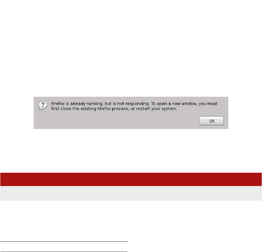
71
A process maps onto a user applicaon (e.g., spreadsheet), a background ulity (e.g., le indexer) or
a system service (e.g., remote login daemon). It is possible that mulple processes might be execung
the same program at once. These would be dierent runme instances of the same program. Some
complex applicaons only permit a single instance of the process to be executed at once. For instance,
the Firefox web browser has a lock le, that prevents mulple instances of the applicaon from
execung with the same user prole, see Figure 4.3.
Figure 4.3: Firefox displays an error message and refuses to run mulple applicaon instances for a single user prole.
4.2.1 Discovering processes
How many processes are execung on your system right now? In an interacve shell session, type:
Lisng 4.2.1: List processes Bash
1 ps aux | wc -l
The ps command displays informaon about processes currently registered with the OS. The opons
we use are as follows:
My Linux server shows 257 processes. How many processes are on your machine? Every me you
invoke a new program, a new process starts. This might occur if you click a program icon in an app
launcher bar, or if you type an executable le name at a shell prompt.
4.2.2 Launching a new process
Let’s nd out how to start a new process programmacally, using the fork system call. This is the
standard Unix approach to create a new process. The fork-ing process (known as the parent) generates
an exact copy (known as the child), that is execung the same code. The only dierence between the
parent and the child (i.e., the only way to disnguish between the two processes) is the return value
of the fork call. In the child process, this return value is 0. In the parent process, the return value is
a posive integer which denotes the allocated process idener (or pid) of the child. Figure 4.4 shows
this sequence schemacally. Note that if we can’t fork a new process, fork returns 1.
a
Include all users’ processes
u
Display user-friendly output
x
Include processes not started from a user terminal
Chapter 4 | Process management
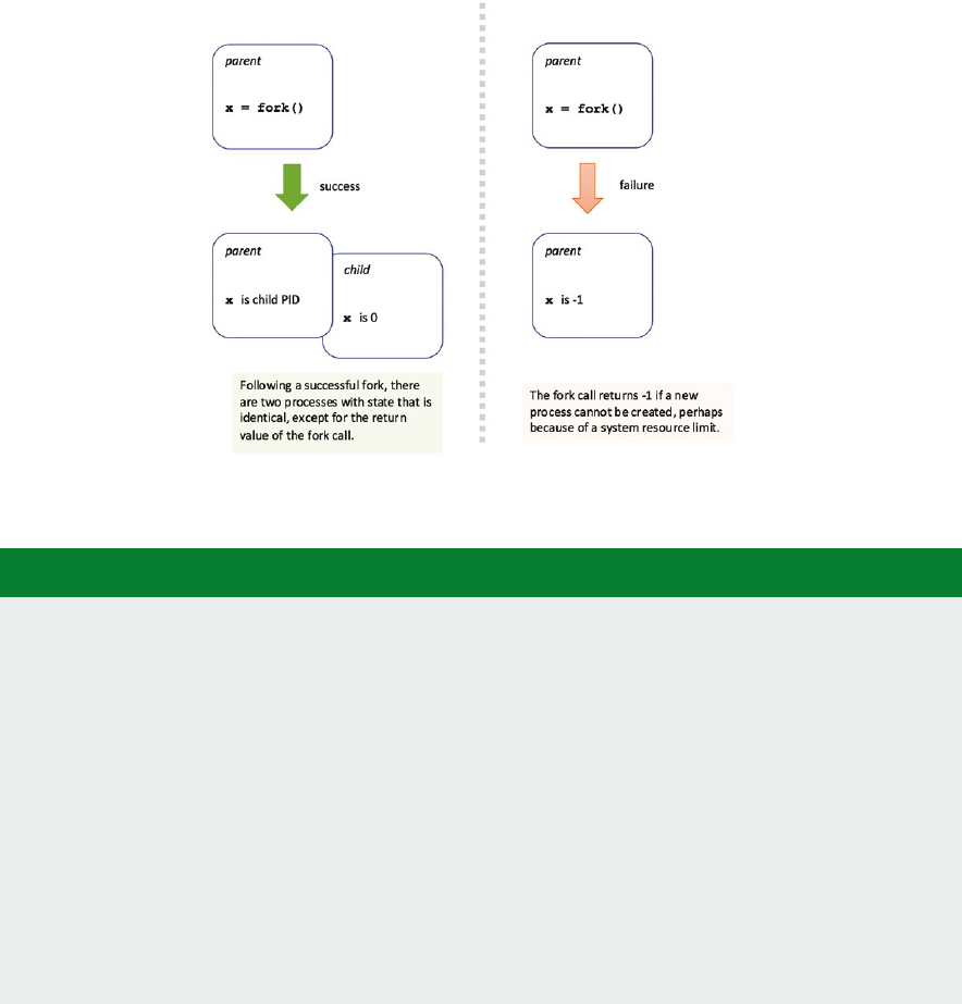
Operang Systems Foundaons with Linux on the Raspberry Pi
72
Below we show a simple Python script. This runs a program that creates a second copy of itself.
Figure 4.4: Schemac diagram of the behavior of the fork system call.
Lisng 4.2.2: Example of fork() in Python Python
1 import os
2
3 def child():
4 print ("Child process has PID {:d}".format(os.getpid()))
5
6 def parent():
7 # only parent executes this code
8 print ("Parent process has PID {:d}".format(os.getpid()))
9 child_pid = os.fork()
10 # both parent and child will execute subsequent if statement
11 if child_pid==0:
12 # child executes this
13 child()
14 else:
15 # parent executes this
16 print ("Parent {:d} has just forked child {:d}".format(
17 os.getpid(), child_pid))
18
19 parent()
The child process is a copy of the parent process, with the only dierence being the return value
of fork. However, the child process occupies an enrely separate virtual address space—so any
subsequent changes made to either the parent or the child memory will not be visible in the other
process. This duplicaon of memory is done in a lazy way, using the copy on write technique to avoid
massive memory copy overheads. Data is shared unl one process (either parent or child) tries to
modify it; then the two processes are each allocated a private copy of that data. Copy on write is
explained in more detail in Secon 6.5.7.

73
4.2.3 Doing something dierent
The fork call allows us to start a new process, but the child is almost exactly a replica of the parent.
How do we execute a dierent program in a child process? Linux supports this with the execve system
call, which replaces the currently running process with data from a specied program binary. The rst
parameter is the name of the executable le, the second parameter is the argument vector (eecvely
argv in C programs), and the third parameter is a set of environment variables, as key/value pairs.
Lisng 4.2.3: Example of execve() in Python Python
1 import os
2
3 os.execve("/bin/ls", ["ls", "-l", "*"], {})
This is precisely how an interacve shell, like bash, launches a new program; rst, the shell calls fork to
start a new process, then the shell calls execve to load the new program binary that the user wants to run.
The execve call does not return unless there is an error that prevents the new program from being
executed. See man execve for details of such errors, in which case execve returns -1. There are
several other variants of execve, which you can nd via man execl.
In Linux, the fork operaon is implemented by the underlying clone system call. The clone funcon
allows the programmer to specify explicitly which parts of the old process are duplicated for the new
process, and which parts are shared between the two processes. A clone call enables the child process
to share parts of its context, such as the virtual address space, with the parent process. This allows us to
support threads as well as processes with a single API, which is the implementaon basis of the Nave
Posix Threads Library (NPTL) in Linux. For instance, the pthread_create funcon invokes the clone
system call. Torvalds [1] gives a descripon of the design raonale for clone.
4.2.4 Ending a process
A parent process can block, waing for a child process to complete. The parent calls the wait funcon
for this purpose. Conversely, a child process can complete by calling the exit funcon with a status
code argument (a non-zero value convenonally indicates an error). Alternavely, the child process
may terminate by returning from its main roune.
The example C code below illustrates the duality between wait in the parent and exit in the child
processes.
Lisng 4.2.4: Example use of wait() in C code C
1 #include <stdio.h>
2 #include <stdlib.h>
3 #include <sys/types.h>
4 #include <sys/wait.h>
5 #include <unistd.h>
6
7 int main() {
Chapter 4 | Process management
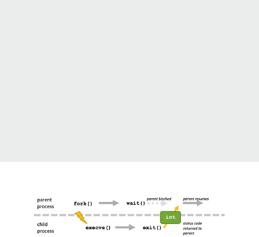
Operang Systems Foundaons with Linux on the Raspberry Pi
74
8
9 pid_t child_pid, pid;
10 int status;
11
12 child_pid = fork();
13
14 if (child_pid == 0) {
15 //child process
16 pid = getpid();
17 printf("I'm child process %d\n", pid);
18 printf("... sleep for 10 seconds, then exit with status 42\n");
19 sleep(10);
20 exit(42);
21 }
22 else if (child_pid > 0) {
23 //parent
24 //waiting for child to terminate
25 pid = wait(&status);
26 if (WIFEXITED(status)) {
27 printf("Parent discovers child exit with status: %d\n", WEXITSTATUS(status));
28 }
29 }
30 else {
31
32 perror("fork failed");
33 exit(1);
34 }
35 return 0;
36 }
Figure 4.5 illustrates the sequence of Linux system calls that are executed by a parent and a child
process during the lifeme of the child.
Figure 4.5: Schemac diagram showing how to start and terminate a child process.
If the parent process completes before the child process, then the child becomes an orphan process.
It is ‘adopted’ by one of the parent’s ancestors, known as a subreaper. See man prctl for details.
If there are no nominated subreapers in the process ancestors, then the child is adopted by the init
process. In either case, the parent eld of the child process’ task_struct is updated when its
original parent exits. This process is known as re-parenng.
4.3 Process metadata
A great deal of informaon is associated with each process. The OS requires this metadata to idenfy,
execute, and manage each process. Generally, the relevant informaon is encapsulated in a data
structure known as a process control block.
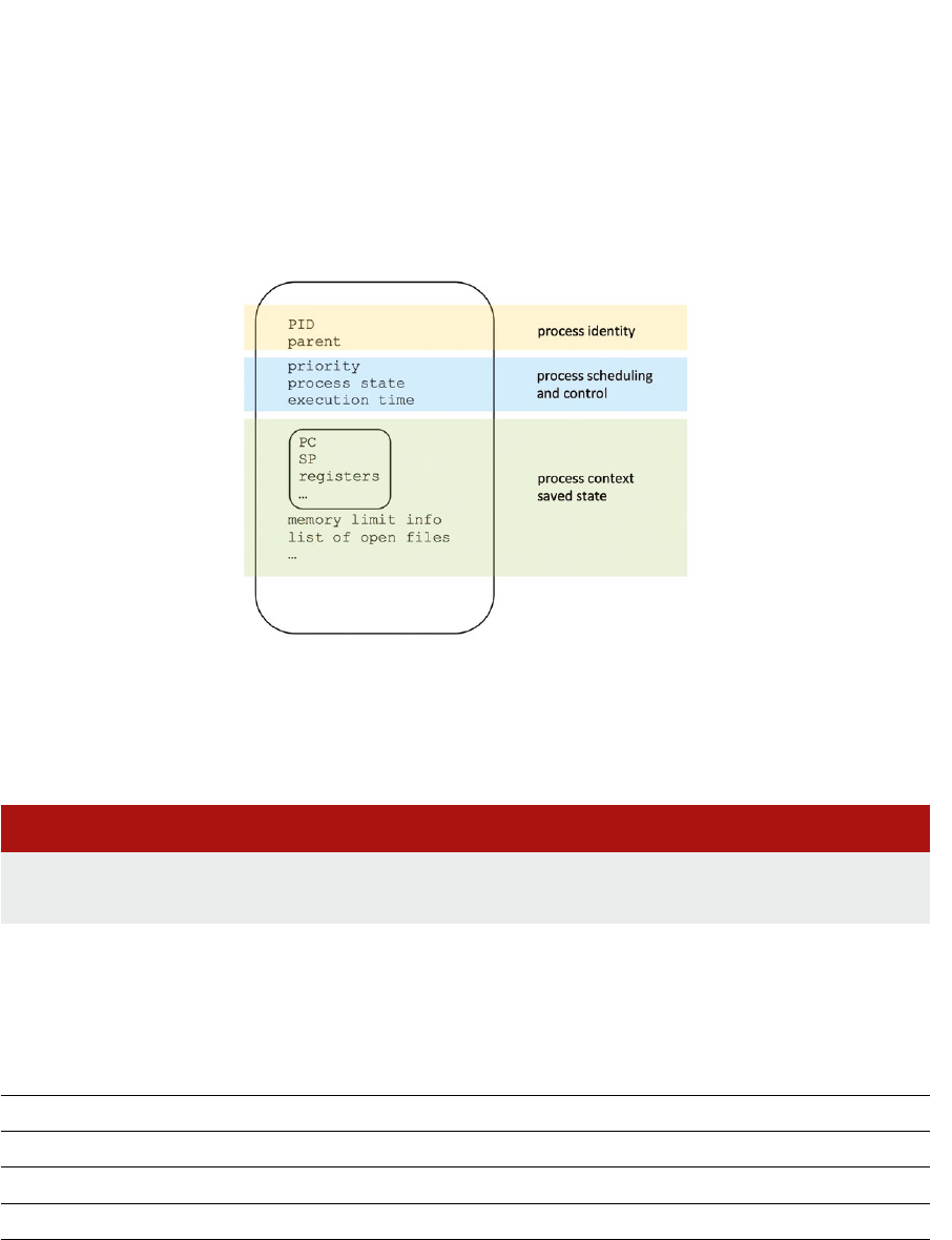
75
The most basic metadata is the unique, posive integer idener associated with a process,
convenonally known as the process pid. Some metadata is related to context switch saved data, such
as register values, open le handles, or memory conguraon. This informaon enables the process to
resume execuon aer it has been suspended by the OS. Further metadata relates to the interacons
between a process and the OS—e.g., proling stascs and scheduling details. Figure 4.6 shows
a high-level schemac diagram of the metadata stored in a process control block.
Figure 4.6: Generic OS management metadata required for each process, stored in a per-process data structure known as the process control block.
4.3.1 The /proc le system
The Linux kernel exposes some process metadata as part of a virtual le system. Let’s look in the
/proc directory on your Linux system:
Lisng 4.3.1: The /proc le system Bash
1 cd /proc
2 ls
You should see a list of directories, many of which will have names that are integers. Each integer
corresponds to a pid, and the les inside these pid directories capture informaon about the relevant
process.
Table 4.1: Virtual les associated with a process in /proc/[pid]/.
cmdline
The textual command that was invoked to start this process
cwd
A symbolic link to the current working directory for this process
exe
A symbolic link to the executable le for this process
fd/
A folder containing le descriptors for each le opened by the process
maps
A table showing how data is arranged in memory
stat
A list of counters for various OS events, specic to this process
Chapter 4 | Process management

Operang Systems Foundaons with Linux on the Raspberry Pi
76
Table 4.1 lists a few of these les and the informaon they contain. For the full list, execute man 5
proc at a Linux terminal prompt. The /proc/[pid] les are not ‘real’—look at the le sizes with
ls -l. These pseudo-les are not stored on the persistent le system: instead, they are le-like
representaons of in-memory kernel metadata for each process.
Let’s list the commands that all the processes in our system are execung:
Lisng 4.3.2: Finding all processes in the system via /proc Bash
1 cd /proc
2 forCMDin`nd.-maxdepth2-name"cmdline"`; do cat $CMD; echo "";done | sort
We observe that some commands are blank—these processes do not have a corresponding command-
line invocaon.
4.3.2 Linux kernel data structures
The Linux kernel spreads process metadata across several linked blocks of memory. In this secon, we
will examine three key data structures:
thread_info
task_struct
thread_struct
The C struct called thread_info is architecture-specic; for the Arm plaorm the struct is dened
in arch/arm/include/asm/thread_info.h. Each thread of execuon has its own unique
thread_info instance, embedded at the base of the thread’s runme kernel stack. (Each thread
has a dedicated 8KB stack in kernel memory for use when execung kernel code; this is disnct from
the regular user-mode stack.) We can extract the thread_info pointer by a low-overhead bitmask
operaon on the stack pointer register, see code below.
Lisng 4.3.3: Snippet from funcon current_thread_info(void) C
1 return (struct thread_info *)
2 (current_stack_pointer & ~(THREAD_SIZE - 1));
The majority of informaon in thread_info relates to the low-level processor context, such as
register values and status ags. The data structure includes a pointer to the corresponding task_-
struct instance for the process.
The C struct called task_struct is the Linux-specic instanaon of the process control block. It is
necessarily a large data structure, storing all the context for the process. The data structure is dened
in the architecture-independent kernel header le linux/sched.h. In the kernel, the C macro
current returns a pointer to the task_struct for the current process. On 32-bit Arm Linux kernel
4.4 the code sizeof(*current) measures the data structure size as 3472 bytes.
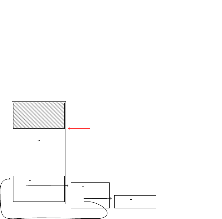
77
The thread_struct data structure is dened in the header le arch/arm/include/asm/
processor.h. This is a small block of memory, referenced by task_struct, which stores more
processor-specic context relang to fault events and debugging informaon.
Each thread has its own unique instances of these three key data structures, although references
to other metadata elements might be shared (e.g., for memory maps or open les, recall the earlier
discussion of the clone system call). Figure 4.7 shows a schemac diagram of these per-thread data
structures and their relaonships.
Figure 4.7: Runme layout of Linux data structures that encapsulate process metadata, residing in kernel memory space.
When a process starts, it runs with a single thread. Its process idener (PID) has the same integer value
as its thread group idener (TGID). If the process creates a new thread, then the new thread shares the
original process address space. The new thread acquires its own PID but retains the original TGID.
As we will see in the next chapter, the Linux scheduler handles all threads in a process as separate
items: in other words, a thread is a kernel-visible schedulable execuon enty, but a process is a user-
visible execuon context. Process tools like top generally merge mulple threads that share a TGID
into a single process.
4.3.3 Process hierarchies
Every process p has a parent, which is the process that created p. The inial system process is the
ancestor of all other processes. In Linux, this is the init process, which has pid 1. The global variable
init_task contains a pointer to the init process’ task_struct.
There are two ways to iterate over processes:
1. Chase the linked list of pointers from one process to the next. This circular doubly-linked list runs
through the processes. Each task_struct instance has a next and prev pointer. The macro
for_each_process iterates overall tasks.
stack frames
thread info
SP
stack grows
down
task struct
thread struct
Chapter 4 | Process management

Operang Systems Foundaons with Linux on the Raspberry Pi
78
2. Chase the linked list of pointers from child process to parent. Each task_struct instance has
a parent pointer. This linear linked list terminates at the init_task.
The C code below will iterate over the linked list from the current task’s process control block to the
init task. It prints out the ‘family tree’ of the processes.
When you invoke this program, how deep is the tree? On my machine, it traverses 5 levels of process
unl it reaches the init process.
Note that this code needs to run in the kernel. It is privileged code since it accesses crical OS data
structures. The easiest way to implement this is to wrap up the code as a kernel module, which is
explained in Secon 2.4.3. The printk funcon is like printf only it outputs to the kernel log,
which you can read with the dmesg ulity.
Lisng 4.3.4: C code to trace a task’s ancestry C
1 #include <linux/module.h> /* Needed by all modules */
2 #include <linux/kernel.h> /* Needed for KERN_INFO */
3 #include <linux/sched.h> /* for task_struct */
4
5 int init_module(void)
6 {
7 struct task_struct *task;
8
9 for (task = current; task != &init_task; task = task->parent) {
10 printk(KERN_INFO " %d (%s) -> ", task->pid, task->comm);
11 }
12 printk(KERN_INFO " %d (%s) \n", task->pid, task->comm);
13
14 return 0;
15 }
In general, it is more ecient to avoid kernel code. Where possible, ulies remain in ‘userland,’ as the
non-kernel code is oen called.
For this reason, most Linux process informaon ulies like ps and top gather process metadata from
the /proc le system, which can be accessed without expensive kernel-level system calls or special
privileges. The pstree tool is another example ulity—it displays similar informaon to our process
family tree code outlined above, but pstree uses the /proc pseudo-les rather than expensive
system calls. The pstree ulity is part of the psmisc Debian package, which you may need to install
explicitly. Figure 4.8 shows typical output from pstree, for a Pi with a single user logged in via ssh.
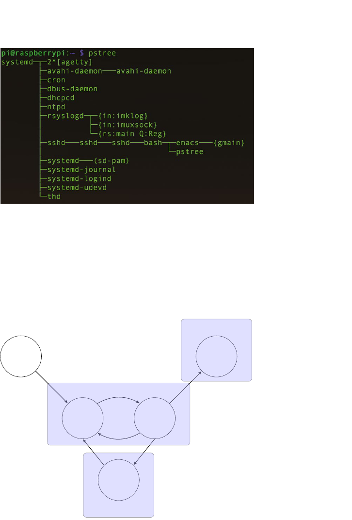
79
Figure 4.8: Process hierarchy output from pstree.
4.4 Process state transions
When a process begins execuon, it can move between various scheduling states. Figure 4.9 shows
a simple state transion diagram, which indicates the state a process might be in, and the acon that
will transfer the process to a dierent state. A more complex version is presented in the next chapter.
Figure 4.9: The state transion diagram for a Linux process, states named in circles, with possible ps state codes indicated.
Table 4.2 lists the dierent process states, and their standard Linux abbreviaons, which you might
see in the output of the ps or top command. Each state corresponds to a bilag value, stored in the
corresponding task->state eld. The values are dened in include/linux/sched.h, which we
explore in more detail in the next chapter.
born
ready
running
dead
waiting
{Z}
{D.S,T}
{R}
Chapter 4 | Process management

Operang Systems Foundaons with Linux on the Raspberry Pi
80
Let’s play with some processes in Linux. Start a process in your terminal, perhaps a text editor like vim.
While it is running, make it stop by pressing CTRL + z. This sends the STOP signal to the process.
Eecvely we have paused its execuon. This is how program debugging works.
Now let’s run another process that incurs heavy disk overhead, perhaps
Table 4.2: Linux process states, see man ps for full details.
Lisng 4.4.1: nd Bash
1 nd/-name"foo" &
or
Lisng 4.4.2: dd Bash
1 dd if=/dev/zero of=/tmp/foo bs=1K count=200K &
Now you can observe your processes with the ps command. Use the watch tool to see how the states
change over me.
Lisng 4.4.3: watch Bash
1 watch ps u
You should see that some processes are running (R) and others are sleeping (S), waing for I/O (D), or
stopped (T). Press CTRL + c to exit the watch program.
A zombie process is a completed child process that is waing to be ‘died up’ by its parent process.
A process remains in the zombie state unl its parent calls the wait funcon, or the parent terminates
itself. The example Python code below will demonstrate a zombie child, as the parent is sleeping for
one minute aer the fork, but the child process exits immediately.
Lisng 4.4.4: Python zombie example Python
1 import os
2 import time
R
Running, or runnable
S
Sleeping, can be interrupted
D
Waing on IO, not interrupble
T
Stopped, generally by a signal
Z
Zombie, a dead process

81
3
4 def main():
5 child_pid = os.fork()
6 # both parent and child will execute subsequent if statement
7 if child_pid==0:
8 # child executes this
9 pid = os.getpid()
10 print ("To see the zombie, run ps u -p {:d}".format(os.getpid()))
11 exit()
12 else:
13 # parent executes this
14 time.sleep(60)
15 print ("Zombie process disappears now")
16
17 main()
4.5 Context switch
The earliest electronic computers were single-tasking. These systems executed one program
exclusively unl another program was loaded into memory. For instance, the early EDSAC machine at
Cambridge would ring a warning bell when a program completed execuon, so the technician could
read o the results and load in a new program. Up unl the 1980s, micro-computers ran single-program
operang systems like DOS and CP/M. For such computers, process management was unnecessary.
Processes are the basis of mul-programming, where the operang system executes mulple
programs concurrently. Eecvely, the operang system mulplexes many processes onto a smaller
number of physical processor cores.
The context switch operaon enables this mulplexing. All the runme data required for a process (as we
outlined in Secon 4.3) is saved into a process control block (eecvely the task_struct in Linux). The
OS serializes the process metadata. Then the process is paused, and another process resumes execuon.
If processes are switched in and out of execuon at suciently high frequency, then it appears that all
the processes are execung simultaneously. This is analogous to a person who is juggling, see Figure
4.10. In the same way, as the OS handles more processes than there are processors, the persons deals
with more juggling balls than s/he has hands.
Figure 4.10: Juggling with more balls than hands is like mul-tasking execuon. Image owned by the author.
Chapter 4 | Process management

Operang Systems Foundaons with Linux on the Raspberry Pi
82
For short-term process scheduling, the process context data is stored in RAM (i.e., kernel memory).
For processes that are not likely to be executed again in the short-term, the process memory is paged
out to disk. Given that the context captures all we need to know to resume the process, this paging
is relavely straighorward (see Chapter 6). Another possibility is that the process might be migrated
across a network link to another machine, perhaps within a cloud datacenter (see Chapter 11).
There are three praccal quesons to ask, in terms of context switching on a Linux system.
Q1: How long does a process actually execute before it is switched out?
We will cover process scheduling in more detail in the next chapter. However, Linux species a
scheduling quantum which is a noonal amount of me each process will be executed in a round-robin
style before a context switch. This quantum me value is specied on my Raspberry Pi as 10ms. You
can check the default value on your Linux system with:
Lisng 4.5.1: Default Linux meslice Bash
1 cat /proc/sys/kernel/sched_rr_timeslice_ms
Q2: How much data do we need to save for a process context?
For each thread, there is a thread_info struct, to capture saved register values and other processor
context. This data structure can be up to around 500 bytes on a 32-bit Arm processor with hardware
oang-point support. There is also process control informaon; however, much of this data will
already be resident in memory, so probably only minor updates required at a context switch event.
Q3: How long does a context switch take, on a standard Linux machine?
The context switch overhead measures the me taken to suspend one process and resume another.
This overhead must be made as low as possible on interacve systems, to enable rapid and smooth
context switching between user processes.
The open-source lmbench ulity [2] contains code to measure a range of low-level system
performance characteriscs, including the context switch overhead. Download the code tarball, then
execute the following commands:
Lisng 4.5.2: Using lmbench Bash
1 tar xvzf lmbench3.tar.gz
2 cd lmbench3/src
3 make results
4 # ignore errors
5 cd ../bin/armv7l-linux-gnu/
6 ./lat_ctx -s 0 10
This reports the context switch overhead for your machine. On my Raspberry Pi 2 Model B v1.1
running Linux kernel 4.4, lmbench reports a context switch overhead of around 12 µs. What do you
measure on your machine?

83
4.6 Signal communicaons
Inter-process communicaon will be covered in a future chapter. For now, we focus only on sending
signals to processes. A signal is like an interrupt — it’s an event generated by the kernel to invoke
a signal handler in another process. Signals are a mechanism for one-way asynchronous nocaons,
with a minimal data payload. The recipient process only knows the signal number and the identy
of the sender. Check out the siginfo_t struct denion in the <sys/siginfo.h> header for
more details.
4.6.1 Sending signals
The simplest way to send a signal to a process is to use the kill command, at a shell prompt, also
specifying the target pid. Below is an example to kill an annoying repeat print loop.
Table 4.3: A selecon of Linux signal codes, consult signal.h for the full set.
Lisng 4.6.1: Example kill process Bash
1 while ((1)) ; do echo "hello $BASHPID"; sleep 5; done &
2 # suppose this prints out hello 15082
3 # ... then you should type
4 kill 15082
Eecvely, this kill command is like interacvely pressing CTRL + c on the console. Study the table
of selected signals below to see some other events that a process may handle and their equivalent
interacve key combinaons.
Note that some signals are standardized across all Unix variants, whereas other signals may be system-
specic. Execute the command man kill or kill -l for details.
Name Number Descripon Interacve
SIGINT
2 Terminal interrupt
CTRL + c
SIGQUIT
3 Terminal quit
SIGILL
4 Illegal instrucon
SIGKILL
9 Kill process (cannot be caught/ignored)
SIGSEGV
11 Segmentaon fault (bad memory access)
SIGPIPE
13 Write on a pipe with no reader, broken pipe
SGALRM
14 Alarm clock Use alarm funcon to set an alarm
SIGCHLD
17 Child process has stopped or exited
SIGCONT
18 Connue execung, if stopped bg or fg
SIGSTOP
19 Stop execung (cannot be caught/ignored)
CTRL + z
Chapter 4 | Process management
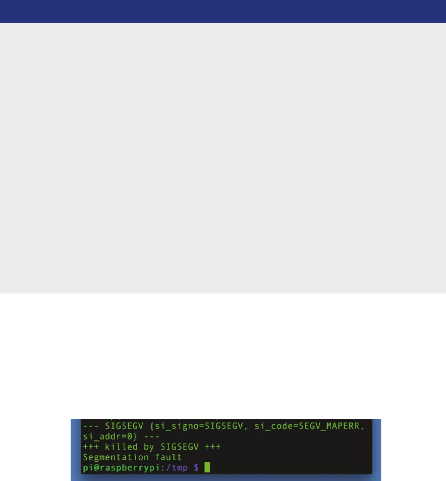
Operang Systems Foundaons with Linux on the Raspberry Pi
84
4.6.2 Handling signals
We have looked at sending signals to processes. Now let’s consider how to handle such signals when
a process receives them. A signal handler is a callback roune which is installed by the process to deal
with a parcular signal. Below is a simple example of a program that responds to the SIGINT signal.
Lisng 4.6.2: Simple signal handler in C C
1 #include <stdio.h>
2 #include <signal.h>
3 #include <string.h>
4 #include <unistd.h>
5
6 struct sigaction act;
7
8 void sighandler(int signum, siginfo_t *info, void *p) {
9 printf("Received signal %d from process %lu\n",
10 signum, (unsigned long)info->si_pid);
11 printf("goodbye\n");
12 }
13
14 int main() {
15 // instructions for interactive user
16 printf("Try kill -2 %lu, or just press CTRL+C\n", (unsigned long)getpid());
17 // zero-initialize the sigaction instance
18 memset(&act, 0, sizeof(act));
19 // set up the callback pointer
20 act.sa_sigaction = sighandler;
21 // set up the ags, so the signal handler receives relevant info
22 act.sa_ags=SA_SIGINFO;
23 // install the handler
24 sigaction(SIGKILL, &act, NULL);
25 // wait for something to happen
26 sleep(60);
27 return 0;
28 }
Some signals cannot be handled by the user process, in parcular, SIGKILL and SIGSTOP. Even if you
aempt to install a handler for these signals, it will never be executed.
If we don’t install a handler for a signal, then the default OS handler is used instead. This will generally
report the signal then cause the process to terminate. For example, consider what happens when your
C programs dereference a null pointer; normally the default SIGSEGV handler supplied by the OS is
invoked, see Figure 4.11.
Figure 4.11 When a program deferences a null pointer, a segmentaon fault occurs and the appropriate OS signal handler reports the error.

85
4.7 Summary
In this chapter, we have explored the concept of a process as a program in execuon. We have seen
how to instanate processes using Linux system calls. We have reviewed the typical lifecycle of
a process and considered the various states in which a process can be found. We have explored the
runme data structures that encapsulate process metadata. Finally, we have seen how to aract the
aenon of a process using the signaling mechanism. Future chapters will explore how processes
are scheduled by the OS and how one process can communicate with other concurrently execung
processes.
4.8 Further reading
O’Reilly’s book on Linux System Programming [3] covers processes from a detailed user code
perspecve. The companion volume on Understanding the Linux Kernel [4] goes into much greater
depth about process management in Linux; although this textbook covers earlier kernel versions,
most of the material is sll directly relevant.
4.9 Exercises and quesons
4.9.1 Mulple choice quiz
1. Which of these is not a mechanism for allowing two processes to communicate with each
another?
a) message passing
b) context switch
c) shared memory
2. What happens when a process receives a signal?
a) The processor switches to privileged mode.
b) Control jumps to a registered signal handler.
c) The process immediately quits.
3. Which of the following items is shared by two threads that are cloned by the same process?
a) thread_info runme metadata
b) program memory
c) call stack
4. Immediately aer a successful fork system call, the only observable dierence between parent
and child processes is:
a) the return value of the fork call
b) the stack pointer
c) the program counter value
Chapter 4 | Process management

Operang Systems Foundaons with Linux on the Raspberry Pi
86
4.9.2 Metadata mix
1. Process metadata may be divided into three dierent kinds: (1) identy, (2) context switch saved
state, and (3) scheduling control informaon. Look at the following elds from the Linux task_
struct data structure in the linux/sched.h header le. For each eld, idenfy which sort of
metadata it is. You may want to look at the comments in the header le for more informaon.
a) unsigned int rt_priority
b) pid_t pid
c) volatile long state;
d) structles_struct*les;
e) void *stack;
f) unsignedlongmaj_t;
4.9.3 Russian doll project
A matryoshka doll is a set of wooden dolls of decreasing size placed one inside another. This challenge
involves creang a matryoshka process. Dene a constant called MATRYOSHKA, and set it to a
small integer value. Now write a C program with a main funcon that sets a local variable x to the
MATRYOSHKA value. Then construct a loop that checks the value of x. If x is less than or equal to 0,
then return, otherwise decrement the value of x and fork a new process. Recall from Secon 4.2 that
the fork call should be wrapped in an if statement to ensure dierent behavior for the parent and
child processes. To make your code more interesng, each individual process could print out its unique
id and its value of x. The output should look like this:
Lisng 4.9.1: Matryoshka program output C
1 " I'm 1173: x is 4 "
2 " I'm 1174: x is 3 "
3 " I'm 1175: x is 2 "
4 " I'm 1176: x is 1 "
5 " I'm 1177: x is 0 "
4.9.4 Process overload
When one user starts too many processes rapidly, the enre system can become unusable. Discuss
why this might happen. Eecvely, rapid process creaon is an OS denial-of-service aack. Search
online for ‘fork-bomb’ aacks to nd out more details [5]. How does the ulimit command migate
such denial-of-service aacks?
4.9.5 Signal frequency
Consider the signals listed in Table 4.3. Which of these signals are likely to be received frequently?
Which signals are rarer? In what circumstances might you use a custom signal handler for your
applicaon?
4.9.6 Illegal instrucons
You can aempt to execute an illegal instrucon on your Raspberry Pi with the assembler code block
shown below:

87
Lisng 4.9.2: Execute an illegal instrucon C
1 int main() {
2 asm volatile (".word 0xe7f0000f\n");
3 return 0;
4 }
Compile this code and execute it. You should see an Illegal Instruction error message. Now
dene a signal handler for SIGILL. At rst, the signal handler should just report the illegal instrucon
and exit the program. As an advanced step, try to get the signal handler to advance the user program
counter by one instrucon (4 bytes) and return. You will need to access and modify the context-
>uc_mcontext.arm_pc data eld.
References
[1] L. Torvalds, The Linux Edge. O’Reilly, 1999, hp://www.oreilly.com/openbook/opensources/book/linus.html
[2] L. W. McVoy, C. Staelin et al., “lmbench: Portable tools for performance analysis.” in USENIX annual technical conference, 1996,
pp. 279–294, download code from hp://www.bitmover.com/lmbench/
[3] R. Love, Linux System Programming: Talking Directly to the Kernel and C Library, 2nd ed. O’Reilly, 2013.
[4] D. P. Bovet and M. Cesa, Understanding the Linux Kernel, 3rd ed. O’Reilly, 2005.
[5] E. S. Raymond, “The new hacker’s diconary: Fork bomb,” 1996, see also hp://www.catb.org/~esr/jargon/html/F/fork-
bomb.html
Chapter 4 | Process management

Chapter 5
Process scheduling

Operang Systems Foundaons with Linux on the Raspberry Pi
90
5.1 Overview
This chapter discusses how the OS schedules processes on a processor. This includes the raonale for
scheduling, the concept of context switching, and an overview of scheduling policies (FCFS, priority, ...)
and scheduler architectures (FIFO, mullevel feedback queues, priories, ...). The Linux scheduler is
studied in detail.
What you will learn
Aer you have studied the material in this chapter, you will be able to:
1. Explain the raonale for scheduling and relaonship to the process lifecycle.
2. Discuss the pros and cons of dierent policies for scheduling in terms of the principles and criteria.
3. Calculate scheduling criteria and reason about scheduling policy performance with respect to the criteria.
4. Analyze the implementaon of scheduling in the Linux kernel.
5. Control scheduling of threads and processes as a programmer or system administrator.
5.2 Scheduling overview: what, why, how?
In Chapter 1, we introduced the concept of tasks and explained what a processor needs to do to allow
mulple tasks to execute concurrently. Each task constutes an amount of work for the CPU, and
scheduling is the method by which this work is assigned to the CPU. The operang system scheduler
is the component responsible for the scheduling acvity.
5.2.1 Denion
According to the Oxford diconary [1], a schedule
1
is “a plan for carrying out a process or procedure,
giving lists of intended events and mes: we have drawn up an engineering schedule”; to schedule
means to “arrange or plan (an event) to take place at a parcular me” or to “make arrangements for
(someone or something) to do something”. In the context of operang systems, both meanings hold:
the scheduler arranges events (i.e., execuon of task code on the CPU) to take place at a parcular
me and makes arrangements for the task to run.
5.2.2 Scheduling for responsiveness
Scheduling is primarily movated by the need to execute mulple tasks concurrently. In a modern
compung system, many tasks are acve at the same me. For example, on a desktop system, every
tab in a web browser is a task; the graphical user interface requires a number of tasks, there are tasks
taking care of networking, etc. At the me of wring this text, my laptop was running 317 processes.
From these, 106 were superuser tasks, 24 were services, and the remaining 190 were owned by my
user account. Most of these tasks are long-running, i.e., they only exit when the system shuts down.
In fact, out of the 190 processes under my user name, only 33 belonged to applicaons that I had
actually launched.
1
The origin is late Middle English (in the sense ‘scroll, explanatory note, appendix’): from Old French cedule, from late Lan schedula ‘slip of paper,’ diminuve of scheda,
from Greek σχεδη ‘papyrus leaf.’

91
Now assume for a moment that the system would execute these tasks one by one, waing unl a task
completes, then execute the next task. The very rst task would occupy the processor forever, so none
of the other tasks would be able to run. Therefore the operang system gives each process, in turn,
a slice of CPU me.
5.2.3 Scheduling for performance
However, there is another important benet of scheduling. The processor is very fast (remember,
even the humble Raspberry Pi executes 10 million instrucons in a single Linux me slice). But
when accessing peripherals for I/O, the processor has to wait for the peripheral, and this can take
a long me because peripherals such as disks are comparavely slow. For example, simply accessing
DRAM without a cache takes between 10 and 100 clock cycles; accessing a hard disk takes several
milliseconds, i.e., millions of clock cycles. Without concurrent execuon, the CPU would idle unl the
I/O request had completed. Instead, the operang system will schedule the next task on the CPU.
5.2.4 Scheduling policies
A scheduling policy is used to decide what share of CPU me a process will get and when it will
be scheduled. In pracce, processes have dierent needs. For example, when playing a video, it is
important that the image does not freeze or stuer, so it is beer to give such a process frequent
short slices than infrequent long slices. On the other hand, many of the system processes that run
invisibly in the background are not ming crical, so the operang system might decide to schedule
them when with low priority.
In the rest of the chapter, we will look in detail at the scheduling component of the kernel and its
relaonship to the process management infrastructure discussed in the previous chapter.
5.3 Recap: the process lifecycle
Recall from the previous chapter that the operang system manages each process through a data
structure called the Process Control Block, which in Linux is implemented using the task_- struct
datastructure. With respect to the process lifecycle, the main aribute of interest is the state which
can be one of the following (from linux/sched.h)
#deneTASK_RUNNING0x0000
#deneTASK_INTERRUPTIBLE0x0001
#deneTASK_UNINTERRUPTIBLE0x0002
#dene__TASK_STOPPED0x0004
#dene__TASK_TRACED0x0008
#deneTASK_PARKED0x0040
#deneTASK_DEAD0x0080
#deneTASK_WAKEKILL0x0100
#deneTASK_WAKING0x0200
#deneTASK_NOLOAD0x0400
#deneTASK_NEW0x0800
#deneTASK_STATE_MAX0x1000
#deneTASK_NORMAL(TASK_INTERRUPTIBLE|TASK_UNINTERRUPTIBLE)
#deneTASK_IDLE(TASK_UNINTERRUPTIBLE|TASK_NOLOAD)
as well as the exit_state which can be one of the following:
Chapter 5 | Process scheduling
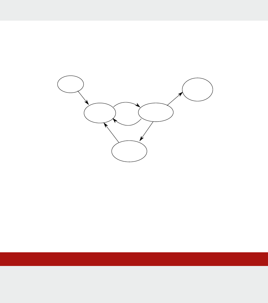
Operang Systems Foundaons with Linux on the Raspberry Pi
92
#deneEXIT_DEAD0x0010
#deneEXIT_ZOMBIE0x0020
Observe that each of these states represents a unique bit in the state value. Figure 5.1 shows the
actual states a process can be in, annotated with the state values. Scheduling is concerned with
moving tasks between these states, in parcular from the run queue to the CPU and from the CPU
to the run queue or the waing state.
Figure 5.1: Linux process lifecycle.
The key point to note is that when the task is running on the CPU, the OS is not running unl an
interrupt occurs. Typically the interrupt is caused by the mer that controls the me slice allocated
to the running process, or raised by peripherals. Another point to note is that most processes actually
spend most of their me in the waing state. This is because most processes frequently perform I/O
operaons (e.g., disk access, network access, keyboard/mouse/touch screen input, ...) and these I/O
operaons usually take a relavely long me to complete. You can check this using the me command,
for example, we can me a command that waits for user input, e.g.
Lisng 5.3.1: Timing a command that waits for user input Bash
1 wim@rpi:~ $ time man man
2
3 real 0m5.275s
4 user 0m0.620s
5 sys 0m0.060s
The man command displays the man page for a command (in this case its own man page) and waits
unl the user hits ’q’ to exit. I hit ’q’ aer about ve seconds.
To interpret the output of the me, we need the denions of real, user, and sys. According to the
man page:
TASK_NEW
TASK_RUNNING
TASK_DEAD
EXIT_DEAD
EXIT_ZOMBIE
TASK_NORMAL
TASK_IDLE
born
(code loaded, PCB created)
ready
(run queue)
running
(on CPU)
waiting
(for I/O, thread sync,...)
died
(PCB still
active)
TASK_RUNNING

93
The me command runs the specied program command with the given arguments. When the
command nishes, me writes a message to standard error giving ming stascs about this program
run. These stascs consist of
the elapsed real me between invocaon and terminaon,
the user CPU me (the sum of the tms_utime and tms_cutime values in a struct tms as returned
by mes(2)), and
the system CPU me (the sum of the tms_stime and tms_cstime values in a struct tms as returned
by mes(2)).
The man page of mes gives us some more details:
The struct tms is as dened in <sys/times.h>:
Lisng 5.3.2: struct tms from <sys/mes.h> C
1 struct tms {
2 clock_t tms_utime; /* user time */
3 clock_t tms_stime; /* system time */
4 clock_t tms_cutime; /* user time of children */
5 clock_t tms_cstime; /* system time of children */
6 };
The tms_utime eld contains the CPU me spent execung instrucons of the calling process. The
tms_stime eld contains the CPU me spent in the system while execung tasks on behalf of the
calling process. The tms_cutime eld contains the sum of the tms_utime and tms_cutime values
for all waited-for terminated children. The tms_cstime eld contains the sum of the tms_stime and
tms_cstime values for all waited-for terminated children.
So what the example tells us is that the process spent only 620 ms out of 5.275 s running user
instrucons and the OS spent 60 ms performing work on behalf of the user process. So for about 4.6
seconds the process was waing for I/O, i.e., the interrupt from the keyboard caused by hing the ’q’
key. Most processes will alternate many mes between running and waing. The me a process spends
in the running state is called the burst me.
5.4 System calls
When a user process wants to perform I/O or any other system-related operaon, it needs to instruct
the operang system to perform the required acon. This operaon is called a system call. Because
the operang system is interrupt-driven, the user process needs to raise a soware interrupt to
give control to the operang system. Furthermore, Linux system calls are idened by a unique
number and take a variable number of arguments. Linux allows us to implement system calls via the
syscall() library funcon (although this is not the used for the common system calls in the C
library). The syscall(2) man page provides a very good discussion of the details. The following secon
gives a summary of the man page, oming specic details for non-Arm architectures.
Chapter 5 | Process scheduling

Operang Systems Foundaons with Linux on the Raspberry Pi
94
5.4.1 The Linux syscall (2) funcon
Lisng 5.4.1: Linux syscall C
1 #dene _GNU_SOURCE /* See feature_test_macros(7) */
2 #include <unistd.h>
3 #include <sys/syscall.h> /* For SYS_xxx denitions */
4 long syscall(long number, ...);
syscall() is a small library funcon that invokes the system call whose assembly language interface
has the specied number with the specied arguments. Employing syscall() is useful, for example,
when invoking a system call that has no wrapper funcon in the C library. syscall() saves CPU
registers before making the system call, restores the registers upon return from the system call, and
stores any error code returned by the system call in errno(3) if an error occurs. Symbolic constants for
system call numbers can be found in the header le <sys/syscall.h>.
The return value is dened by the system call being invoked. In general, a 0 return value indicates
success. A −1 return value indicates an error, and an error code is stored in errno.
Architecture calling convenons
Each architecture ABI (Applicaon Binary Interface) has its own requirements on how system call
arguments are passed to the kernel. For system calls that have a glibc wrapper (e.g., most system
calls), glibc handles the details of copying arguments to the right registers in a manner suitable for the
architecture.
Every architecture has its own way of invoking and passing arguments to the kernel. The details for the
(32-bit) EABI and arm64 (i.e., AArch64) architectures are listed in the two tables below.
Table 5.1 lists the instrucon used to transion to kernel mode (which might not be the fastest or best way
to transion to the kernel, so you might have to refer to vdso(7)), the register used to indicate the system
call number, the register used to return the system call result, and the register used to signal an error.
Table 5.1: Instrucon used to transion to kernel mode.
Table 5.2 shows the registers used to pass the system call arguments.
Table 5.2: Registers used to pass the system call arguments.
ABI Instrucon Syscall# Retval Error
arm/EABI swi #0 r7 r0 -
arm64 svc #0 x8 x0 -
ABI arg1 arg2 arg3 arg4 arg5 arg6 arg7
arm/EABI r0 r1 r2 r3 r4 r5 r6
arm64 x0 x1 x2 x3 x4 x5 x-

95
The Cortex-A53 is an AArch64 core which supports both ABIs. However, the Raspbian Linux shipped
with the Raspberry Pi 3 is a 32-bit Linux, so it uses the EABI. This means that it uses swi (Soware
Interrupt) rather than svc (Supervisor Call) to perform a system call. However, in pracce, they are
synonyms, and their purpose is to provide a mechanism for unprivileged soware to make a system
call to the operang system. The X* registers in AArch64 indicated that the general-purpose R*
registers are accessed as 64-bit registers. [2]
For example (taken from the syscall man page), using syscall(), the readahead() system call would be
invoked as follows on the Arm architecture with the EABI in lile-endian mode:
Lisng 5.4.2: Example syscall: readahead() C
1 syscall(SYS_readahead, fd, 0,
2 (unsigned int)(oset&0xFFFFFFFF),
3 (unsigned int)(oset>>32),
4 count);
5.4.2 The implicaons of the system call mechanism
Whenever a user process wants to perform I/O or any other system-related operaon, the operang
system takes over. This means that every system call involves a context switch, with overheads,
as discussed in the previous chapter. Note that in the me taken to perform a context switch me
(around 10µs) the CPU could have executed 10,000 operaons, so the overhead of context switching
is considerable.
Virtual dynamic shared object (vDSO)
To reduce the overhead of system calls, over me two mechanisms have been introduced
into the Linux kernel: vsyscall (virtual system call) and vDSO Dynamic Shared Object). The
original vsyscall mechanism is now obsolete so we only discuss the vDSO. The purpose of
both mechanism is the same: to allow system calls without the need for a context switch.
The raonale behind this mechanism is that some system calls that are frequently used do
not actually require kernel privileges, and therefore handing control over these operaons to
the kernel is an unnecessary overhead. As the name indicates, these calls are implemented
in a special dynamically shared library (linux-vdso.so) which is automacally provided by the
kernel to any process created. In pracce, for the Arm architecture only two system calls are
implemented this way: clock_geme() and gemeofday().
5.5 Scheduling principles
Aer this detour into the process lifecycle and the role of system calls, let’s have a look at the
principles of OS scheduling and what criteria an OS can use to make scheduling decisions.
Let’s assume a number of tasks are acve in the system, and that each of these tasks spends a certain
poron of its lifeme running on the CPU and another poron waing. It is also possible that the task
is ready to run, but the CPU is occupied by another task.
Chapter 5 | Process scheduling
Operang Systems Foundaons with Linux on the Raspberry Pi
96
5.5.1 Preempve versus non-preempve scheduling
A rst design decision to make is if the scheduler will be able to interrupt running tasks, for example,
to run a task that it considers more important (i.e., it has a higher priority). If this is the case, the
scheduler is called pre-empve. In Linux, all scheduling is preempve. The opposite, non-preempve
scheduling, can be used if the tasks voluntarily yield the CPU to other tasks. This is called cooperave
multasking and is not commonly used in modern operang systems.
Note that we do not use the term preempon when a task is moved to the waing state because
this is not a scheduling acvity. From a scheduling perspecve, the remainder of the task can be
considered as a new task (belonging to the same process or thread).
5.5.2 Scheduling policies
The scheduling policy is the approach to scheduling taken by the scheduler. To understand the concept
beer, consider that the scheduler must keep a list of tasks that are ready to run. This list is ordered in
some way, and the task at the head of the list is the one that will run next. Therefore the main decision of
the scheduler is in which posion in the list to put a new ready task. Furthermore, the scheduler must also
decide for how long a task can run if it is not pre-empted by another task or interrupted by a system call.
Essenally, these two decisions form the scheduling policy. Linux has several dierent scheduling policies,
each task (i.e., each process or thread) can be set to one of these policies. The praccal implementaon
of a policy is an algorithm, so somemes we will use the term scheduling algorithm instead.
5.5.3 Task aributes
We menoned above (Secon 5.5.1) that the scheduler can consider one task more important than
another, and therefore give a higher priority of execuon to the more important task. This means that
the more important task can either be run sooner, or for longer, or both. The importance of a task
depends on its aributes. A task aribute could, for example, be the me when the task was put in the
task list, or its posion in the task list; or the me it takes for the task to run; or the amount of CPU
me that has already been spent by the task. Or the task can have an explicit priority aribute, which
in pracce is a small integer value used by the kernel to assess how important a process is.
The Linux kernel uses several of the above-menoned aributes, depending on the scheduling policy
used, and all threads have a priority aribute.
5.6 Scheduling criteria
When selecng a scheduling policy, we can use dierent criteria, e.g., depending on the typical
process mix on the system, or depending on the requirements on the threads in an applicaon.
The most commonly used criteria are:
CPU ulizaon: Ideally, the CPU would be busy 100% of the me, so that we don’t waste any CPU cycles.
Throughput: The number of processes completed per unit me.
Turnaround me: The elapsed (wall clock) me required for a parcular task to complete, from birth
me to death.

97
Waing me: The me spent by a task in the ready queue waing to be run on the CPU.
Response me: The me taken between subming a request and obtaining a response.
Load average: The average number of processes in the ready queue. On Linux, it is reported by
"upme" and "who."
In general, we want to opmize the average value of criteria, i.e., maximize CPU ulizaon and
throughput, and minimize all the others. It is also desirable to minimize the variance of a criteria
because users prefer a consistently predictable system over an inconsistent one, even if the laer
performs beer on average.
5.7 Scheduling policies
In this secon, we discuss some common scheduling policies that make it easier to understand the
actual design choices and implementaon details are for the Linux kernel scheduler. To analyze the
behavior and performance of the various scheduling algorithms we use a Gan chart, i.e., a simple plot
of the task id on a discrete meline. Table 5.3 shows the example task conguraon that will be used
to create the Gan charts for the dierent scheduling policies.
Table 5.3: Example task conguraon.
5.7.1 First-come, rst-served (FCFS)
This is a very simple scheduling policy where the aribute deciding its priority is simply its relave
arrival me in the list of runnable tasks. In this context, this lists is a FIFO queue called the run queue.
The scheduler simply takes the task at the head of the queue and runs it on the CPU unl it either
nishes or gets interrupted by a system call and hence moves to the waing state. When the tasks
have nished waing, it will be re-added at the tail of the run queue. FCFS scheduling can either be
preempve or non-preempve, as illustrated in Figures 5.2 and 5.3.
Figure 5.2: Schedule for the example task conguraon with non-preempve FCFS.
Pid Burst me Arrival me Priority
1 12 0 0
2 6 2 1
3 2 4 1
4 4 8 2
5 8 16 0
6 8 20 1
7 2 20 0
8 10 24 0
FCFS,non-preemptive
time
0
2
4
6
8
10
12
14
16
18
20
22
24
26
28
30
32
34
36
38
40
arrival
1
2
3
4
5
6,7
8
run
1
1
1
1
1
1
2
2
2
3
4
4
5
5
5
5
6
6
6
6
7
Chapter 5 | Process scheduling

Operang Systems Foundaons with Linux on the Raspberry Pi
98
Figure 5.3: Schedule for the example task conguraon with preempve FCFS.
5.7.2 Round-robin (RR)
Round robin is another very simple scheduling policy that is nevertheless very widely used. We
introduced it already in Chapter 1. This policy consists of running every task for a xed amount of
me.This amount of me is known as the me slice or scheduling quantum. The choice of the quantum
is crucial: if it is too long, the system will become unresponsive; if it is too short, the context switching
overhead will be considerable. As menoned in the previous chapter, you can check this value on your
Linux system using:
Lisng 5.7.1: Linux round-robin quantum from /proc Bash
1 cat /proc/sys/kernel/sched_rr_timeslice_ms
On the Raspberry Pi 3, it is 10 ms.
The schedule for the example task conguraon using RR is shown in Figure 5.4.
Figure 5.4: Schedule for the example task conguraon with Round-Robin scheduling.
5.7.3 Priority-driven scheduling
In priority-driven scheduling, the order in the run queue is determined by the priority of the process
or thread; in other words, the run queue is a priority queue. In general, we can observe the following:
A priority-driven scheduler is an on-line scheduler.
It does NOT precompute a schedule of tasks/jobs.
It assigns priories to jobs when they are released and places them on a ready job queue
in priority order.
When preempon is allowed, a scheduling decision is made whenever a job is released
or completed.
At each scheduling decision me, the scheduler updates the ready job queue and then schedules
and executes the job at the head of the queue.
FCFS,preemptive
time
0
2
4
6
8
10
12
14
16
18
20
22
24
26
28
30
32
34
36
38
40
arrival
1
2
3
4
5
6,7
8
run
1
1
2
3
4
4
1
1
5
5
6
6
8
8
8
8
8
1
1
2
2
time 0 2 4 6 8 10 12 14 16 18 20 22 24 26 28 30 32 34 36 38 40
arrival 1 2 3 4
5 6,7 8
run 112234415566788112556
RR,q=4

99
We can disnguish between xed-priority and dynamic-priority algorithms:
A xed-priority algorithm assigns the same priority to all the jobs in a task.
A dynamic-priority algorithm assigns dierent priories to the individual jobs in a task.
The priority of a job is usually assigned upon its release and does not change. The next two example
scheduling policies use me-related informaon as the priority.
5.7.4 Shortest job rst (SJF) and shortest remaining me rst (SRTF)
If we knew how long it would take for a task to run, we could reorder the run queue so that the
shortest task would be at the head of the queue. This policy is called shortest job rst (SJF) or
somemes shortest job next, and an illustrave schedule is shown in Figure 5.5. I menon it because
it is a very common one in other textbooks, e.g. [3], but it is not very praccal as in general the
scheduler can’t know how long a task will take to complete. It is, however, the simplest example of
the use of a task aribute as a priority (the priority is inverse to the predicted remaining CPU me).
Furthermore, SJF is provably opmal, in that for a given set of tasks and their execuon mes, it gives
the least average waing me for each process.
Figure 5.5: Schedule for the example task conguraon with Shortest Job First scheduling.
The preempve version of SJF is called shortest remaining me rst (SRTF). The criterion for
preempon, in this case, is that a newly arrived task has a shorter remaining run me than the
currently running task (Figure 5.6). This policy has been proven to be the opmal preempve policy
[4]. Both SJF and SRTF have an addional drawback: it is possible that some tasks will never run unl
because their remaining me is always considered to be longer than that of any other task in the
system. This is known as starvaon.
Figure 5.6: Schedule for the example task conguraon with Shortest Remaining Time First scheduling.
Figure 5.7: Schedule for the example task conguraon with Shortest Elapsed Time First scheduling.
SJF
time 0 2 4 6 8 10 12 14 16 18 20 22 24 26 28 30 32 34 36 38 40
arrival 1 2 3 4
5 6,7 8
run 1111113442227555
56666
SRTF
time 0 2 4 6 8 10 12 14 16 18 20 22 24 26 28 30 32 34 36 38 40
arrival 1 2 3 4
5 6,7 8
run 123224415555766661111
SETF
time 0 2 4 6 8 10 12 14 16 18 20 22 24 26 28 30 32 34 36 38 40
arrival 1 2 3 4
5 6,7 8
run 123144215566888887255
Chapter 5 | Process scheduling
Operang Systems Foundaons with Linux on the Raspberry Pi
100
5.7.5 Shortest elapsed me rst (SETF)
SJF and SRTF are so-called clairvoyant algorithms, as they require the scheduler to know informaon
that is not available, in this case, the remaining run me of the process. A more praccal approach is
to use the elapsed run me of a process instead, which is of course easily measurable by the OS. The
paper “Speed Is as Powerful as Clairvoyance” [5] proved that SETF not only obtains good average-case
response me but also does not starve any job.
5.7.6 Priority scheduling
The term “priority scheduling” is used for priority-driven scheduling where the priority of the task is an
enrely separate aribute, not related to other task aributes. Priority driven scheduling can either be
preempve or non-preempve, as illustrated in Figures 5.8 and 5.9.
Figure 5.8: Schedule for the example task conguraon with non-preempve Priority scheduling.
Figure 5.9: Schedule for the example task conguraon with preempve Priority scheduling.
The advantage of using a separate priority rather than, e.g. a me-based aribute of the task is that
the priority can be changed if required. This is essenal to prevent starvaon, as menoned for SJF.
Any priority-based scheduling policy carries the risk that low-priority processes may never execute
because there is always a higher-priority process taking precedence. To remedy this, the priority
should not be stac but increased with the age of the process. This is called aging.
5.7.7 Real-me scheduling
Real-me applicaons are applicaons that process data in real-me, i.e., without delays. From a
scheduling perspecve, this means that the tasks have well dened me constraints. Processing must
be done within the dened constraints to be considered correct, in parcular, not nishing a process
within a given deadline can cause incorrect funconality.
We can disnguish two types of real-me systems:
So real-me systems give no guarantee as to when a crical real-me process will be scheduled,
but only guarantee that the crical process will have a higher priority. A typical example is video and
audio stream processing: missing deadlines will aect the quality of the playback bit is not fatal.
In hard real-me systems, a task must be serviced by its deadline, so the scheduler must be able to
guarantee this. This is, for example, the case for the controls of an airplane or other safety-crical
systems.
Priority,non-preemptive
time 0 2 4 6 8 10 12 14 16 18 20 22 24 26 28 30 32 34 36 38 40
arrival 1 2 3 4
5 6,7 8
run 111111222555578888836
Priority,preemptive
time 0 2 4 6 8 10 12 14 16 18 20 22 24 26 28 30 32 34 36 38 40
arrival 1 2 3 4
5 6,7 8
run 1111112255557888
88366

101
5.7.8 Earliest deadline rst (EDF)
The Linux kernel supports both types of real-me scheduling. For so real-me scheduling, it uses
Round-Robin or FIFO. For hard real-me scheduling, it uses an algorithm known as Earliest Deadline
First (EDF). This is a dynamic priority-driven scheduling algorithm for periodic tasks, i.e., tasks that
periodically need some work to be done. This periodic acvity is usually called a job. The period and
the deadline for the jobs of each task must be known.
The job queue is ordered by the earliest deadline of the jobs. To compute this deadline, the scheduler
must be aware of the period of each task, the phase dierences between those periods and the
execuon mes and deadlines for each job. Usually, the deadline is the same as the period, i.e.,
a job for a given task must nish within one period. In that case, each task can be described by a tuple
(phase, period, execuon me).
Algorithm 5.1 EDF Schedule for example tasks T1 = (0,2,1), T2 = (0,5,2.5)
Time Ready to Run Scheduled
0 J1,1[2]; J2,1[5] J1,1
1 J2,1[5] J2,1
2 J1,2[4]; J2,1[5] J1,2
3 J2,1[5] J2,1
4 J2,1[5]; J1,3[6] J2,1
4.5 J1,3[6] J1,3
5 J1,3[6]; J2,2[10] J1,3
5.5 J2,2[10] J2,2
6 J1,4[8]; J2,2[10] J1,4
7 J2,2[10] J2,2
8 J1,5[10]; J2,2[10] J1,5
9 J2,2[10] J2,2
For example, consider a system with two tasks which both started at me t=0, so the phase is 0 for both.
T1 has a period of 2 and an execuon me of 1; T2 has a period of 5 and an execuon me of 2.5:
T1 = (0 , 2, 1)
T2 = (0 , 5, 2.5)
In other words, both tasks are acve half of the me, so in principle together, they will use the CPU
100%. Because the tasks are periodic, it is sucient to calculate a schedule for the least common
mulple of the periods of T1 and T2, in this task 2*5=10. The schedule is shown below. This is an
important property of EDF: it guarantees that all deadlines are met provided that the total CPU
ulizaon is not more than 100%. In other words, it is always possible to create a valid schedule.
5.8 Scheduling in the Linux kernel
The Linux kernel supports two categories of scheduling, normal and real-me. A good explanaon
is provided in the sched(7) man page. With regards to scheduling, the thread is the main abstracon,
i.e., the scheduler schedules threads rather than processes.
Each thread has an associated scheduling policy and a stac scheduling priority. The scheduler makes its
decisions based on knowledge of the stac scheduling policy and priority of all threads in the system.
Chapter 5 | Process scheduling

Operang Systems Foundaons with Linux on the Raspberry Pi
102
There are currently (kernel 4.14) three normal scheduling policies: SCHED_OTHER, SCHED_IDLE and
SCHED_BATCH, and three real-me policies, SCHED_FIFO, SCHED_RR and SCHED_DEADLINE. Of these,
SCHED_OTHER, SCHED_FIFO and SCHED_RR are required by the POSIX 1003.1b real-me standard [6].
For threads scheduled using one of the normal policies, the stac priority is not used in scheduling decisions
(it is set to 0). Processes scheduled under one of the real-me policies have a stac priority value in the
range 1 (low) to 99 (high). Thus real-me threads always have higher stac priority than normal threads.
The scheduler maintains a list of runnable threads per stac priority value. To determine which thread
to run next, it looks for the non-empty list with the highest stac priority and selects the thread at the
head of this list.
The scheduling policy determines where a thread is to be inserted into the list of threads with equal
priority and how it will progress to the head of the list.
In Linux, all scheduling is preempve: if a thread with a higher stac priority becomes ready to run,
the currently running thread will be pre-empted and returned to the run list for its priority level. The
scheduling policy of the thread determines the ordering within the run list. This means that, e.g. for
the run list with stac priority 0, i.e., the normal scheduling category (SCHED_- NORMAL), there can
be up to three dierent policies that decide the relave ordering of the threads. For each of the higher
stac priority run lists (real-me), there can be one or two.
5.8.1 User priories: niceness
Niceness or nice value is the relave, dynamic priority of a process. Niceness values range from
-20 (most favorable to the process) to 19 (least favorable to the process) and the value aects how
the process is scheduled, but not in a direct way. The nice value of a running process can be changed
by the user via the nice(1) command or the nice(2) system call. We will see further how the dierent
schedulers use these values. Note that nice values are only for non-real-me processes.
5.8.2 Scheduling informaon in the task control block
As menoned before, the task control block is implemented in the Linux kernel in the task_struct
data structure, dened in include/linux/sched.h. Let’s have a look at the scheduling-specic informaon
stored in the task_struct (all other elds have been removed for conciseness).
Lisng 5.8.1: task_struct from <include/linux/sched.h> C
1 struct task_struct {
2
3 int on_rq;
4 /** - int prio, static_prio;
5 priority of a process used when scheduled. Variable prio, which is the
6 user-nice values can be converted to static priority to better scale
7 various scheduler parameters.
8 */
9 int prio, static_prio, normal_prio;
10 unsigned int rt_priority; // for soft real-time
11
12 const struct sched_class *sched_class; // see below

103
13 struct sched_entity se; // see below
14 struct sched_rt_entity rt; // for soft real-time
15 struct sched_dl_entity dl; // for hard real-time
16
17 /** the scheduling policy used for this process, as listed above */
18 unsigned int policy;
19 };
This structure includes a number of other scheduling-related data structures. We will discuss sched_
entity and the real-me variants sched_rt_entity and sched_dl_entity. in the secons on the
CFS and real-me schedulers. The sched_class struct is eecvely an interface for the actual scheduling
class in use: all funconality is implemented in each of the separate scheduling classes fair, idle,rt,deadline.
Lisng 5.8.2: sched_class from <include/linux/sched.h> C
1 struct sched_class {
2 const struct sched_class *next;
3
4 void (*enqueue_task) (struct rq *rq, struct task_struct *p, intags);
5 void (*dequeue_task) (struct rq *rq, struct task_struct *p, intags);
6 void (*yield_task) (struct rq *rq);
7 bool (*yield_to_task)
8 (struct rq *rq, struct task_struct *p, bool preempt);
9
10 void (*check_preempt_curr)
11 (structt rq *rq, struct task_struct *p, intags);
12
13 struct task_struct * (*pick_next_task)
14 (struct rq *rq,struct task_struct *prev,structrq_ags*rf);
15 void (*put_prev_task) (struct rq *rq, struct task_struct *p);
16
17 void (*set_curr_task) (struct rq *rq);
18 void (*task_tick) (struct rq *rq, struct task_struct *p, int queued);
19 void (*task_fork) (struct task_struct *p);
20 void (*task_dead) (struct task_struct *p);
21
22 void (*switched_from) (struct rq *this_rq, struct task_struct *task);
23 void (*switched_to) (struct rq *this_rq, struct task_struct *task);
24 void (*prio_changed)
25 (struct rq *this_rq, struct task_struct *task,int oldprio);
26
27 unsigned int (*get_rr_interval) (struct rq *rq,
28 struct task_struct *task);
29
30 void (*update_curr) (struct rq *rq);
31
32 };
So in order to perform a scheduling operaon for a process p, all the scheduler has to do is call
p->sched_class-><name of the operation>
and the corresponding operaon for the parcular scheduling class for that process will be carried out.
The Linux kernel keeps a per-CPU runqueue (struct rq) which contains dierent runqueues per
scheduling class as follows (from sched.h):
Chapter 5 | Process scheduling

Operang Systems Foundaons with Linux on the Raspberry Pi
104
Lisng 5.8.3: runqueue struct from <include/linux/sched.h> C
1 / *
2 * This is the main, per-CPU runqueue data structure.
3 *
4 */
5 struct rq {
6 / * runqueue lock: */
7 raw_spinlock_t lock;
8 unsigned int nr_running;
9 #dene CPU_LOAD_IDX_MAX 5
10 unsigned long cpu_load[CPU_LOAD_IDX_MAX];
11 struct load_weight load;
12 unsigned long nr_load_updates;
13 u64 nr_switches;
14 struct cfs_rq cfs;
15 struct rt_rq rt;
16 struct dl_rq dl;
17 struct task_struct *curr, *idle, *stop;
18 };
5.8.3 Process priories in the Linux kernel
The kernel uses the priories as set or reported by nice() and as stac priories and represents them
on a scale from 0 to 139. Priories from 0 to 99 are reserved for real-me processes and 100 to 139
(which are the nice values from -20 through to +19 shied by 120) are for normal processes. The
kernel code implemenng this can be found in include/linux/sched/prio.h, together with some macros
to convert between nice values and priories.
Lisng 5.8.4: Linux kernel priority calculaon C
1 #dene MAX_NICE 19
2 #dene MIN_NICE -20
3 #dene NICE_WIDTH (MAX_NICE - MIN_NICE + 1)
4
5 / *
6 * Priority of a process goes from 0..MAX_PRIO-1, valid RT
7 * priority is 0..MAX_RT_PRIO-1, and SCHED_NORMAL/SCHED_BATCH
8 * tasks are in the range MAX_RT_PRIO..MAX_PRIO-1. Priority
9 * values are inverted: lower p->prio value means higher priority.
10 *
11 * The MAX_USER_RT_PRIO value allows the actual maximum
12 * RT priority to be separate from the value exported to
13 * user-space. This allows kernel threads to set their
14 * priority to a value higher than any user task. Note:
15 * MAX_RT_PRIO must not be smaller than MAX_USER_RT_PRIO.
16 */
17
18 #dene MAX_USER_RT_PRIO 100
19 #dene MAX_RT_PRIO MAX_USER_RT_PRIO
20
21 #dene MAX_PRIO (MAX_RT_PRIO + NICE_WIDTH)
22 #dene DEFAULT_PRIO (MAX_RT_PRIO + NICE_WIDTH / 2)
23
24 / *
25 * Convert user-nice values [ -20 ... 0 ... 19 ]
26 * to static priority [ MAX_RT_PRIO..MAX_PRIO-1 ],

105
27 * and back.
28 */
29 #dene NICE_TO_PRIO(nice) ((nice) + DEFAULT_PRIO)
30 #dene PRIO_TO_NICE(prio) ((prio) - DEFAULT_PRIO)
31
32 / *
33 * 'User priority' is the nice value converted to something we
34 * can work with better when scaling various scheduler parameters,
35 * it's a [ 0 ... 39 ] range.
36 */
37 #dene USER_PRIO(p) ((p)-MAX_RT_PRIO)
38 #dene TASK_USER_PRIO(p) USER_PRIO((p)->static_prio)
39 #dene MAX_USER_PRIO (USER_PRIO(MAX_PRIO))
Priority info in task_struct
The task_struct contains several priority-related elds:
int prio, static_prio, normal_prio;
unsigned int rt_priority; // for soft real-time
stac_prio is the priority set by the user or by the system itself:
p->static_prio = NICE_TO_PRIO(nice_value);
normal_priority is based on stac_prio and on the scheduling policy of a process, i.e., real-me or
“normal” process. Tasks with the same stac priority that use dierent policies will get dierent normal
priories. Child processes inherit the normal priories.
p->prio is the so-called “dynamic priority.” It is called dynamic because it can be changed by the system,
for example when the system temporarily raises a task’s priority to a higher level, so that it can preempt
another high-priority task. Inially, prio is set to the same value as stac_prio. The actual dynamic
priority is computed as:
p->prio=eective_prio(p);
This funcon, dened in kernel/sched/core.c, returns the normal_prio unless the task is a real-me
task, in which case it uses normal_prio() to recompute the normal priority
Lisng 5.8.5: Implementaon of eecve_prio() C
1 static int eective_prio(struct task_struct *p)
2 {
3 p->normal_prio = normal_prio(p);
4 / *
5 * If we are RT tasks or we were boosted to RT priority,
6 * keep the priority unchanged. Otherwise, update priority
7 * to the normal priority:
8 */
9 if (!rt_prio(p->prio))
Chapter 5 | Process scheduling

Operang Systems Foundaons with Linux on the Raspberry Pi
106
10 return p->normal_prio;
11 return p->prio;
12 }
For a real-me task, it calculates normal_prio as
Lisng 5.8.6: Implementaon of normal_prio() C
1 static inline int normal_prio(struct task_struct *p)
2 {
3 int prio;
4 if (task_has_dl_policy(p))
5 prio = MAX_DL_PRIO-1;
6 else if (task_has_rt_policy(p))
7 prio = MAX_RT_PRIO-1 - p->rt_priority;
8 else
9 prio = p->static_prio;
10 return prio;
11 }
In other words, if the task is not real-me, then prio, stac_prio, and normal_prio have the same value.
Priority and load weight
The way the priories are used is not simply to order tasks but to compute a “load weight,” which is
then used to calculate the CPU me allowed for a task.
The structure task_struct->se.load contains the weight of a process in a struct load_weight:
Lisng 5.8.7: load_weight struct C
1 struct load_weight {
2 unsigned long weight;
3 u32 inv_weight;
4 };
The weight is roughly equivalent to 1024/(1.25)^(nice), the actual values are hardcoded in the array
sched_prio_to_weight (in kernel/sched/core.c):
Lisng 5.8.8: Scheduling priority-to-weight conversion C
1 const int sched_prio_to_weight[40] = {
2 /* -20 */ 88761, 71755, 56483, 46273, 36291,
3 /* -15 */ 29154, 23254, 18705, 14949, 11916,
4 /* -10 */ 9548, 7620, 6100, 4904, 3906,
5 /* -5 */ 3121, 2501, 1991, 1586, 1277,
6 /* 0 */ 1024, 820, 655, 526, 423,
7 /* 5 */ 335, 272, 215, 172, 137,
8 /* 10 */ 110, 87, 70, 56, 45,
9 /* 15 */ 36, 29, 23, 18, 15,
10 };

107
This conversion is used in set_load_weight
Lisng 5.8.9: Implementaon of set_load_weight() C
1 static void set_load_weight(struct task_struct *p)
2 {
3 int prio = p->static_prio - MAX_RT_PRIO;
4 struct load_weight *load = &p->se.load;
5 /*
6 * SCHED_IDLE tasks get minimal weight:
7 */
8 if (idle_policy(p->policy)) {
9 load->weight = scale_load(WEIGHT_IDLEPRIO);
10 load->inv_weight = WMULT_IDLEPRIO;
11 return;
12 }
13 load->weight = scale_load(sched_prio_to_weight[prio]);
14 load->inv_weight = sched_prio_to_wmult[prio];
15 }
Here scale_load is a macro which increases resoluon on 64-bit architectures; SCHED_IDLE is a
scheduler policy for very low priority system background tasks. The inv_weight eld is used to speed
up reverse computaons. So in essence, the operaon is
load->weight = sched_prio_to_weight[prio];
The way the weight is used depends on the scheduling policy.
5.8.4 Normal scheduling policies: the completely fair scheduler
All normal scheduling policies in the Linux kernel (SCHED_OTHER, SCHED_IDLE, and SCHED_BATCH) are
implemented as part of what is known as the “Completely Fair Scheduler” (CFS). The philosophy behind this
scheduler, which was introduced in kernel version 2.6.23 in 2009, is stated in the kernel documentaon
(hps://elixir.bootlin.com/linux/latest/source/kernel/sched/sched.h) as follows:
80% of CFS’s design can be summed up in a single sentence: CFS basically models an “ideal, precise mul-
tasking CPU” on real hardware.
“Ideal mul-tasking CPU” is a (non-existent :-)) CPU that has 100% physical power and which can run each
task at precise equal speed, in parallel, each at 1nr_running speed. For example: if there are 2 tasks running,
then it runs each at 50% physical power --- i.e., actually in parallel.
On real hardware, we can run only a single task at once, so we have to introduce the concept of “virtual
runme.” The virtual runme of a task species when its next meslice would start execuon on the ideal
mul-tasking CPU described above. In pracce, the virtual runme of a task is its actual runme normalized
to the total number of running tasks.
In other words, the CFS aempts to balance the virtual runme overall tasks. The CFS scheduler run
queue (struct cfs_rq cfs in struct rq in sched.h) is a priority queue with the task with the
smallest virtual runme at the head of the queue.
Chapter 5 | Process scheduling

Operang Systems Foundaons with Linux on the Raspberry Pi
108
Lisng 5.8.10: Implementaon of CFS runqueue C
1 /* CFS-related elds in a runqueue */
2 struct cfs_rq {
3 struct load_weight load;
4 unsigned long runnable_weight;
5 unsigned int nr_running, h_nr_running;
6 u64 exec_clock;
7 u64 min_vruntime;
8 struct rb_root_cached tasks_timeline;
9 / *
10 * 'curr' points to currently running entity on this cfs_rq.
11 * It is set to NULL otherwise (i.e., when none are currently running).
12 */
13 struct sched_entity *curr, *next, *last, *skip;
14 };
The CFS algorithm computes the duraon of the next me slice for this task based on the priories of
all tasks in the queue and runs it.
The calculaon of the virtual runme is done in the funcons sched_slice(), sched_- vslice()
and calc_delta_fair() in fair.c, using informaon from the sched_enty struct se:
Lisng 5.8.11: sched_enty struct for calculaon of virtual runme C
1 struct sched_entity {
2 /* For load-balancing: */
3 struct load_weigh load;
4 struct rb_node run_node;
5 struct list_head group_node;
6 unsigned int on_rq;
7
8 u64 exec_start;
9 u64 sum_exec_runtime;
10 u64 vruntime;
11 u64 prev_sum_exec_runtime;
12
13 u64 nr_migrations;
14
15 struct sched_statistics statistics;
16
17 };
As the actual C code in the kernel is quite convoluted, below we present equivalent Python code:
Lisng 5.8.12: Calculaon of virtual runme slice Python
1 # Targeted preemption latency for CPU-bound tasks.
2 # NOTE: this latency value is not the same as the concept of 'timeslice length'
3 # - timeslices in CFS are of variable length and have no persistent notion
4 # like in traditional, time-slice based scheduling concepts.
5 sysctl_sched_latency = 6 ms * (1 + ilog(ncpus))
6 # Minimal preemption granularity for CPU-bound tasks:
7 sysctl_sched_min_granularity = 0.75 ms * (1 + ilog(ncpus))
8 sched_nr_latency = sysctl_sched_latency/sysctl_sched_min_granularity #6/0.75=8

109
9
10 def sched_slice(cfs_rq, tasks):
11 se =head(tasks)
12 # The idea is to set a period (slice) in which each task runs once.
13 # When there are too many tasks (sched_nr_latency)
14 # we have to stretch this period because otherwise, the slices get too small.
15 nrr = cfs_rq.nr_running + (not se.on_rq)
16 slice = sysctl_sched_latency
17 if nrr > sched_nr_latency:
18 slice = nrr * sysctl_sched_min_granularity
19 # slice is scaled using the weight of every other task in the run queue
20 for se in tasks:
21 cfs_rq = cfs_rq_of(se)
22 if not se.on_rq:
23 cfs_rq.load.weight += se.load.weight
24 slice = slice*se.load.weight/cfs_rq.load.weight
25 return slice
26
27
28 # The vruntime slice of a to-be-inserted task is: vslice = slice / weight
29
30 def calc_delta_fair(slice,task):
31 return slice*1024/task.load.weight
32
33 def sched_vslice(cfs_rq, tasks):
34 slice = sched_slice(cfs_rq, tasks)
35 se = head(tasks)
36 vslice = calc_delta_fair(slice,se)
37 return vslice
The actual posion of a task in the queue depends on vrunme, which is calculated as follows:
Lisng 5.8.13: Calculaon of vrunme Python
1 # Update the current task's runtime statistics.
2 def update_min_vruntime(cfs_rq):
3 curr = cfs_rq.curr
4 leftmost=rb_rst_cached(cfs_rq.tasks_timeline)
5 vruntime = cfs_rq.min_vruntime
6 if curr:
7 if curr.on_rq:
8 vruntime = curr.vruntime
9 else:
10 curr = None
11
12 if leftmost: /* non-empty tree */
13 se = rb_entry(leftmost)
14 if not curr:
15 vruntime = se.vruntime
16 else:
17 vruntime = min_vruntime(vruntime, se.vruntime)
18
19 # ensure we never gain time by being placed backwards.
20 cfs_rq.min_vruntime = max_vruntime(cfs_rq.min_vruntime, vruntime)
21
22 def update_curr(cfs_rq):
23 curr = cfs_rq.curr
24 now = rq_clock_task(rq_of(cfs_rq))
25 delta_exec = now - curr.exec_start
26 curr.exec_start = now
27 curr.sum_exec_runtime += delta_exec
Chapter 5 | Process scheduling

Operang Systems Foundaons with Linux on the Raspberry Pi
110
28 curr.vruntime += calc_delta_fair(delta_exec,curr)
29 cfs_rq = update_min_vruntime(cfs_rq)
30
31 def update_curr_fair(rq):
32 update_curr(cfs_rq_of(rq.curr.se))
In other words, the kernel calculates the dierence between the me the process started (exec_- start)
and the current me (now) and then updates exec_start to now. Then it uses this delta_exec and
the load weight to calculate vrunme. Finally, the min_vrunme is calculated as the minimum of the
vrunme of the task at the head of the queue (i.e., the lemost node in the red-black tree) and the
vrunme of the current task. The code checks if there is a current task, and if the queue is not empty
and provides fallbacks. This calculated value is then compared with the currently stored value (cfs_
rq.min_vrunme) and the largest of the two becomes the new cfs_rq.min_vrunme.
5.8.5 So real-me scheduling policies
The Linux kernel supports both so real-me scheduling policies SCHED_RR and SCHED_FIFO
required by the POSIX real-me specicaon [7]. Real-me processes are managed by a separate
scheduler, dened in <kernel/sched/rt.c>.
From the kernel’s perspecve, real-me processes have one key dierence compared to other
processes: if there is a runnable real-me task, it will be run—unless there is another real-me task
with a higher priority.
There are currently two scheduling policies for so real-me tasks:
SCHED_FIFO: This is a First-Come. First-Served scheduling algorithm as discussed in Secon
5.7.1. Tasks following this policy do not have meslices; they run unl they block, yield the CPU
voluntarily or get pre-empted by a higher priority real-me task. A SCHED_FIFO task must have
a stac priority > 0 so that it always preempts any SCHED_NORMAL, SCHED_BATCH or SCHED_
IDLE process. Note that this means that a SCHED_FIFO task will use the CPU unl it nished, and
no non-real-me tasks will be scheduled on that CPU. Several SCHED_FIFO tasks of the same
priority run round-robin. A task can be pre-empted by a higher-priority task, in which case it will
stay at the head of the list for its priority and will resume execuon as soon as all tasks of higher
priority are blocked again. When a blocked SCHED_FIFO thread becomes runnable, it will be
inserted at the end of the list for its priority.
SCHED_RR: This is a Round-Robin (as explained in Secon 5.7.2) enhancement of SCHED_FIFO
scheduler, so it runs every task for a maximum xed me slice. Tasks of the same priority run round-
robin unl pre-empted by a more important task. If aer running for a me quantum, a task is not
nished, it will be put at the end of the list for its priority. A task that has been pre-empted by a
higher priority task and subsequently resumes execuon will complete the remaining poron of its
round-robin me quantum. As menoned before, the length of the me quantum can be retrieved
via /proc/sys/kernel/sched_rr_timeslice_ms or by using sched_rr_get_interval(2).

111
The kernel gives real-me tasks a stac priority, which does not get dynamically recalculated; the only
way to change this priority is by using the chrt(1) command. This ensures that a real-me task always
preempts a normal one and that strict order is kept between real-me tasks of dierent priories.
So real-me processes use a separate scheduling enty struct sched_rt_enty (rt in the task_struct):
Lisng 5.8.14: So real-me scheduling enty struct C
1 struct sched_rt_entity {
2 struct list_head run_list;
3 unsigned long timeout;
4 unsigned long watchdog_stamp;
5 unsigned int time_slice;
6 unsigned short on_rq;
7 unsigned short on_list;
8
9 struct sched_rt_entity *back;
10 #ifdef CONFIG_RT_GROUP_SCHED
11 struct sched_rt_entity *parent;
12 /* rq on which this entity is (to be) queued: */
13 struct rt_rq *rt_rq;
14 /* rq "owned" by this entity/group: */
15 struct rt_rq *my_q;
16 #endif
17 };
As explained in Secon 5.8.2, the main runqueue contains dedicated runqueues for the normal (CFS),
so real-me (rt) and hard real-me (dl) scheduling classes. The so real-me queue uses a priority
queue implemented using a stac array of linked lists and a bitmap. All real-me tasks of a given
priority prio are kept in a linked list in active.queue[prio] and a bitmap (active.bitmap),
keeps track of whether a parcular queue is empty or not.
Lisng 5.8.15: So real-me runqueue C
1 /* Real-Time classes' related eld in a runqueue: */
2 struct rt_rq {
3 struct rt_prio_array active;
4 unsigned int rt_nr_running;
5 unsigned int rr_nr_running;
6 #if dened CONFIG_SMP || dened CONFIG_RT_GROUP_SCHED
7 struct {
8 int curr; /* highest queued rt task prio */
9 } highest_prio;
10 #endif
11 int rt_queued;
12
13 int rt_throttled;
14 u64 rt_time;
15 u64 rt_runtime;
16 /* Nests inside the rq lock: */
17 raw_spinlock_t rt_runtime_lock;
18
19 #ifdef CONFIG_RT_GROUP_SCHED
20 unsigned long rt_nr_boosted;
21
22 struct rq *rq;
Chapter 5 | Process scheduling

Operang Systems Foundaons with Linux on the Raspberry Pi
112
23 struct task_group *tg;
24 #endif
25 };
26
27 / *
28 * This is the priority-queue data structure of the RT scheduling class:
29 */
30 struct rt_prio_array {
31 DECLARE_BITMAP(bitmap, MAX_RT_PRIO+1); /* include 1 bit for delimiter */
32 struct list_head queue[MAX_RT_PRIO];
33 };
34
35 struct rt_bandwidth {
36 /* nests inside the rq lock: */
37 raw_spinlock_t rt_runtime_lock;
38 ktime_t rt_period;
39 u64 rt_runtime;
40 struct hrtimer rt_period_timer;
41 unsigned int rt_period_active;
42 };
Similar to update_curr() in the CFS, there is an update_curr_rt() funcon, dened in kernel/
sched/rt.c in real-me scheduler. This funcon keeps track of the CPU me spent by so real-
me tasks, collects some stascs, updates meslices where needed, and calls the scheduler when
appropriate. All calculaons are done using actual me; no virtual clock is used.
5.8.6 Hard real-me scheduling policy
Since kernel version 3.14 of the Linux kernel (2014), Linux supports hard real-me scheduling via the
SCHED_DEADLINE scheduling class. This is an implementaon of the Earliest Deadline First (EDF)
algorithm discussed in Secon 5.7.8, combined with the Constant Bandwidth Server (CBS) algorithm [8].
According to the sched(7) Linux manual page:
The SCHED_DEADLINE (sporadic task model deadline scheduling) policy is currently implemented using
GEDF (Global Earliest Deadline First) in conjuncon with CBS (Constant Bandwidth Server). A sporadic task
is one that has a sequence of jobs, where each job is acvated at most once per period. Each job also has
a relave deadline, before which it should nish execuon, and a computaon me, which is the CPU me
necessary for execung the job. The moment when a task wakes up because a new job has to be executed is
called the arrival me. The start me is the me at which a task starts its execuon. The absolute deadline
is thus obtained by adding the relave deadline to the arrival me.
A SCHED_DEADLINE task is guaranteed to receive a given runme every period, and this runme
is available within deadline from the beginning of the period.
The runme, period, and deadline are stored in the struct sched_dl_enty struct (dl in the task_
struct) and can be set using the sched_setar() system call:

113
Lisng 5.8.16: Hard real-me scheduling enty struct C
1 struct sched_dl_entity {
2 /* the node in the red-black tree.
3 The red-black tree is used as priority queue
4 */
5 struct rb_node rb_node;
6
7 / *
8 * Original scheduling parameters.
9 */
10 u64 dl_runtime; /* Maximum runtime for each instance */
11 u64 dl_deadline; /* Relative deadline of each instance */
12 u64 dl_period; /* Separation of two instances (period) */
13 u64 dl_bw; /* dl_runtime / dl_period */
14 u64 dl_density; /* dl_runtime / dl_deadline */
15
16 / *
17 * Actual scheduling parameters. Initialized with the values above,
18 * they are continuously updated during task execution.
19 */
20 s64 runtime; /* Remaining runtime for this instance */
21 u64 deadline; /* Absolute deadline for this instance */
22 unsigned int ags;/* Specifying the scheduler behavior */
23
24 / *
25 * Some bool ags
26 */
27 unsigned int dl_throttled : 1;
28 unsigned int dl_boosted : 1;
29 unsigned int dl_yielded : 1;
30 unsigned int dl_non_contending : 1;
31
32 / *
33 * Per-task bandwidth enforcement timer.
34 */
35 struct hrtimer dl_timer;
36
37 / *
38 * Inactive timer
39 */
40 struct hrtimer inactive_timer;
41 };
Time budget allocaon
When a task wakes up because a new job has to be executed (i.e., at arrival me), deadline and
runtime are recalculated as follows (this is the Constant Bandwidth Server or CBS algorithm [8]):
if deadline < currentTime or
runme
> dl_runme then
deadline—currentTime dl_period
deadline = currentTime+dl+deadline
runtime = dl_runtime
else deadline and runme are le unchanged.
Chapter 5 | Process scheduling

Operang Systems Foundaons with Linux on the Raspberry Pi
114
This calculaon is done in setup_new_dl_enty in kernel/sched/deadline.c:
Lisng 5.8.17: Deadline and runme recalculaon C
1 static inline void setup_new_dl_entity(struct sched_dl_entity *dl_se)
2 {
3 struct dl_rq *dl_rq = dl_rq_of_se(dl_se);
4 struct rq *rq = rq_of_dl_rq(dl_rq);
5
6 if (dl_se->dl_throttled)
7 return;
8
9 dl_se->deadline = rq_clock(rq) + dl_se->dl_deadline;
10 dl_se->runtime = dl_se->dl_runtime;
11 }
This funcon is called via
enqueue_task_dl()
g
enqueue_dl_entity()
g
eupdate_dl_entity()
As explained in Secon 5.7.8, the EDF algorithm selects the task with the smallest deadline like the
one to be executed rst. In other words, we have a priority queue where the deadline is the priority.
Just like for the CFS, in the kernel, this priority queue is implemented using a red-black tree. The
lemost node in the tree has the smallest deadline and is cached so that selecng this node is O(1).
When a task executes for an amount of me ∆t, its runme is decreased as
runme = runme − ∆t
This is done in update_curr_dl in kernel/sched/deadline.c:
Lisng 5.8.18: Runme update for EDF scheduling C
1 static void update_curr_dl(struct rq *rq)
2 {
3 struct task_struct *curr = rq->curr;
4 struct sched_dl_entity *dl_se = &curr->dl;
5 u64 delta_exec;
6
7 if (!dl_task(curr) || !on_dl_rq(dl_se))
8 return;
9
10 delta_exec = rq_clock_task(rq) - curr->se.exec_start;
11 if (unlikely((s64)delta_exec <= 0)) {
12 return;
13 }
14
15 dl_se->runtime -= delta_exec;
16
17 throttle:
18 if (dl_runtime_exceeded(dl_se) ) {
19 dl_se->dl_throttled = 1;
20 __dequeue_task_dl(rq, curr, 0);
21 if (unlikely(dl_se->dl_boosted || !start_dl_timer(curr)))
22 enqueue_task_dl(rq, curr, ENQUEUE_REPLENISH);

115
23
24 if (!is_leftmost(curr, &rq->dl))
25 resched_curr(rq);
26 }
27
28 if (rt_bandwidth_enabled()) {
29 struct rt_rq *rt_rq = &rq->rt;
30
31 raw_spin_lock(&rt_rq->rt_runtime_lock);
32 if (sched_rt_bandwidth_account(rt_rq))
33 rt_rq->rt_time += delta_exec;
34 raw_spin_unlock(&rt_rq->rt_runtime_lock);
35 }
36 }
This funcon is called via
scheduler_tick()
g
task_tick_dl()
g
update_curr_dl()
When the runme becomes less than or equal to 0, the task cannot be scheduled unl its deadline.
The CBS feature in the kernel throles tasks that aempt to over-run their specied runme. This
is done by seng a mer for the replenishment of the me budget to the deadline (start_dl_
timer(curr)).
When this replenishment me is reached, the budgets are updated:
deadline = currentTime+dl+deadline
runtime = dl_runtime
5.8.7 Kernel preempon models
User space programs are always preempble. However, in certain real-me scenarios, it may be
desirable to preempt kernel code as well.
The Linux kernel provides several preempon models, which have to be selected when compiling
the kernel. For hard real-me performance, the “Fully Preempble Kernel” preempon model must
be selected. The last two entries below are available only with the PREEMPT_RT patch set. This is an
ocial kernel patch set which gives the Linux kernel hard real-me capabilies. We refer to HOWTO
setup Linux with PREEMPT_RT properly for more details. The possible preempon models are detailed
in the kernel conguraon le kernel/Kcong.preempt:
No Forced Preempon (Server): The tradional Linux preempon model, geared towards
throughput. System call returns and interrupts are the only preempon points.
Voluntary Kernel Preempon (Desktop): This opon reduces the latency of the kernel by adding
more “explicit preempon points” to the kernel code at the cost of slightly lower throughput.
In addion to explicit preempon points, system call returns and interrupt returns are implicit
preempon points.
Chapter 5 | Process scheduling

Operang Systems Foundaons with Linux on the Raspberry Pi
116
Preempble Kernel (Low-Latency Desktop): This opon reduces the latency of the kernel by making
all kernel code (that is not execung in a crical secon) preempble. An implicit preempon point
is located aer each preempon disables secon.
Preempble Kernel (Basic RT): This preempon model resembles the “Preempble Kernel (Low-
Latency Desktop)” model. Besides the properes menoned above, threaded interrupt handlers
are forced (as when using the kernel command line parameter threadirqs). This model is mainly used
for tesng and debugging of substuon mechanisms implemented by the PREEMPT_RT patch.
Fully Preempble Kernel (RT): All kernel code is preempble except for a few selected crical
secons. Threaded interrupt handlers are forced. Furthermore, several substuon mechanisms,
like sleeping spinlocks and rt_mutex are implemented to reduce preempon disabled secons.
Addionally, large preempon disabled secons are substuted by separate locking constructs.
This preempon model has to be selected in order to obtain real-me behavior.
5.8.8 The red-black tree in the Linux kernel
The Linux kernel uses a red-black tree as the implementaon of its priority queues. The red-black tree
is a self-balancing binary search tree with O(log(n)) guarantees on accessing (search), inseron and
deleon of node. More specically, the height H of a red-black tree with n nodes (the length of the
path from the root to the deepest node in the tree) is bounded by:
log (n + 1) ≤ H ≤ 2log (n + 1)
The implementaon of the red-black tree in the linux kernel is lib/rbtree.c, the API is include/linux/
rbtree.h and the data structure is documented in rbtree.txt. The API is quite simple, as illustrated by
example in the documentaon:
Creang a new rbtree
Data nodes in a rbtree tree are structures containing a struct rb_node member:
Lisng 5.8.19: Node in a rbtree C
1 struct mytype {
2 struct rb_node node;
3 char *keystring;
4 };
When dealing with a pointer to the embedded struct rb_node, the containing data structure may be
accessed with the standard container_of() macro. In addion, individual members may be accessed
directly via rb_entry(node, type, member).
At the root of each rbtree is a rb_root structure, which is inialized to be empty via:
Lisng 5.8.20: Root for rbtree C
1 struct rb_root mytree = RB_ROOT;

117
Searching for a value in a rbtree
Wring a search funcon for your tree is fairly straighorward: start at the root, compare each value,
and follow the le or right branch as necessary.
Example:
Lisng 5.8.21: Search funcon for rbtree C
1 struct mytype *my_search(struct rb_root *root, char *string)
2 {
3 struct rb_node *node = root->rb_node;
4
5 while (node) {
6 struct mytype *data = container_of(node, struct mytype, node);
7 int result;
8
9 result = strcmp(string, data->keystring);
10
11 if (result < 0)
12 node = node->rb_left;
13 else if (result > 0)
14 node = node->rb_right;
15 else
16 return data;
17 }
18 return NULL;
19 }
Inserng data into a rbtree
Inserng data in the tree involves rst searching for the place to insert the new node, then inserng
the node and rebalancing ("recoloring") the tree. The search for inseron diers from the previous
search by nding the locaon of the pointer on which to gra the new node. The new node also needs
a link to its parent node for rebalancing purposes.
Example:
Lisng 5.8.22: Inseron in rbtree C
1 int my_insert(struct rb_root *root, struct mytype *data)
2 {
3 struct rb_node **new = &(root->rb_node), *parent = NULL;
4
5 /* Figure out where to put new node */
6 while (*new) {
7 struct mytype *this = container_of(*new, struct mytype, node);
8 int result = strcmp(data->keystring, this->keystring);
9
10 parent = *new;
11 if (result < 0)
12 new = &((*new)->rb_left);
13 else if (result > 0)
14 new = &((*new)->rb_right);
15 else
16 return FALSE;
17 }
18
19 /* Add new node and rebalance tree. */
Chapter 5 | Process scheduling

Operang Systems Foundaons with Linux on the Raspberry Pi
118
20 rb_link_node(&data->node, parent, new);
21 rb_insert_color(&data->node, root);
22
23 return TRUE;
24 }
Removing or replacing exisng data in a rbtree
To remove an exisng node from a tree, call:
Lisng 5.8.23: Removal from rbtree C
1 void rb_erase(struct rb_node *victim, struct rb_root *tree);
Example:
Lisng 5.8.24: Removal from rbtree – example C
1 struct mytype *data = mysearch(&mytree, "walrus");
2
3 if (data) {
4 rb_erase(&data->node, &mytree);
5 myfree(data);
6 }
To replace an exisng node in a tree with a new one with the same key, call:
Lisng 5.8.25: Replace node in rbtree C
1 void rb_replace_node(struct rb_node *old, struct rb_node *new,
2 struct rb_root *tree);
Replacing a node this way does not re-sort the tree: If the new node doesn’t have the same key as the
old node, the rbtree will probably become corrupted.
Iterang through the elements stored in a rbtree (in sort order)
Four funcons are provided for iterang through a rbtree’s contents in sorted order. These work on
arbitrary trees, and should not need to be modied or wrapped (except for locking purposes):
Lisng 5.8.26: Iterate through rbtree C
1 struct rb_node *rb_rst(struct rb_node *tree);
2 struct rb_node *rb_last(struct rb_node *tree);
3 struct rb_node *rb_next(struct rb_node *node);
4 struct rb_node *rb_prev(struct rb_node *node);

119
To start iterang, call rb_rst() or rb_last() with a pointer to the root of the tree, which will return
a pointer to the node structure contained in the rst or last element in the tree. To connue, fetch the
next or previous node by calling rb_next() or rb_prev() on the current node. This will return NULL when
there are no more nodes le.
The iterator funcons return a pointer to the embedded struct rb_node, from which the containing
data structure may be accessed with the container_of() macro, and individual members may be
accessed directly via rb_entry(node, type, member).
Example:
Lisng 5.8.27: Iterate through rbtree – example C
1 struct rb_node *node;
2 for(node=rb_rst(&mytree);node;node=rb_next(node))
3 printk("key=%s\n", rb_entry(node, struct mytype, node)->keystring);
Cached rbtrees
An interesng feature of the Linux implementaon of the red-black tree is caching. Because compung
the lemost (smallest) node in a red-black tree is quite a common task, the cached rbtree rb_root_cached
can be used to opmize O(logN) rb_rst() calls to an O(1) simple pointer fetch, avoiding potenally
expensive tree iteraons. The runme overhead for maintenance is negligible, and the memory footprint
is only slightly larger: a cached rbtree is simply a regular rb_root with an extra pointer to cache the
lemost node. Consequently, any occurrence of rb_root can be substuted by rb_root_cached.
5.8.9 Linux scheduling commands and API
There are a number of commands that allow users to set and change process priories for both normal
and real-me tasks.
Normal processes
The nice command allows the user to set the priority of the process to be executed:
Lisng 5.8.28: Use of the nice command Bash
1 $ nice -n 12 command
The renice command allows to change the priority of a running process:
Lisng 5.8.29: Use of the renice command Bash
1 $ renice -n 15 -p pid
Remember that nice values range from -20 to 19 and lower nice values correspond to higher priority.
So, -12 has a higher priority than 12. The default nice value is 0. Regular users can set lower priories
(posive nice values).To use higher priories (negave nice values), superuser privileges are required.
Chapter 5 | Process scheduling

Operang Systems Foundaons with Linux on the Raspberry Pi
120
Real-me processes
There is a single command to control the real-me properes of a process, chrt. This command sets
or retrieves the real-me scheduling aributes of a running process or runs the command with the
given aributes. The are a number of ags that allow us to set the scheduling policy (–other, –fo,–rr,
–batch, –idle, –deadline).
For example:
Lisng 5.8.30: Use of the chrt command Bash
1 $ chrt --batch 0 pwd
All real-me policies require superuser privileges, for example:
Lisng 5.8.31: Use of the chrt command Bash
1 $ sudo chrt --rr 32 pwd
The –deadline policy only works with sporadic tasks that have actual runme, deadline, and period
aributes set via the sched_setar system call.
5.9 Summary
In this chapter, we have introduced the concept of scheduling, the raonale behind it, and how it
relates to the process life cycle and to the concept of system calls. We have discussed the dierent
scheduling principles and criteria and covered a number of scheduling policies, both the basic policies
and the more advanced policies used in the Linux kernel, including so and hard real-me scheduling
policies. Then we have applied all this basic scheduling theory in a study of the Linux scheduler,
covering the actual data structures and algorithms used by the dierent schedulers supported by
the Linux kernel, the Completely Fair Scheduler, the so real-me scheduler, and the hard real-me
scheduler.
5.10 Exercises and quesons
5.10.1 Wring a scheduler
For this exercise, we suggest you start from exisng code provided in the tutorial series Bare-Metal
Programming on Raspberry Pi 3 on GitHub. Start from the provided cyclic execuve example.
1. Create a round-robin scheduler.
2. Create a FIFO scheduler.
5.10.2 Scheduling
1. What are the reasons for having an operang systems scheduler?
2. How does scheduling relate to the process lifecycle?

121
5.10.3 System calls
1. What is the raonale behind system calls?
2. What are the implicaons of the system call mechanism on scheduling?
5.10.4 Scheduling policies
1. What are the criteria for evaluang the suitability of a given scheduling policy?
2. Consider the following set of processes, with the arrival me and burst me given in milliseconds:
It is assumed below that a process arriving at me t is added to the Ready Queue before a scheduling
decision is made.
a) Draw three Gan charts that illustrate the execuon of these processes using the following
scheduling algorithms: FCFS, preempve priority (a smaller priority number implies a higher priority),
and RR (quantum = 1).
b) The best possible turnaround me for a process is its CPU burst me – i.e., that it is scheduled
immediately upon arrival and runs to compleon without being pre-empted. We will call the dierence
of the turnaround me, and the CPU burst me the excess turnaround me. Which of the algorithms
results in the minimum average excess turnaround me?
3. Discuss the similaries and dierences between the Shortest job rst (SJF), Shortest remaining me
rst (SRTF) and Shortest elapsed me rst (SETF) scheduling policies.
5.10.5 The Linux scheduler
1. How are priories used in the Completely Fair Scheduler?
Explain the use of the Red-Black tree in the Completely Fair Scheduler.
Discuss the policies for so and hard real-me scheduling in the Linux kernel.
Process Arrival Time Burst Time Priority
P1 0 10 3
P2 1 1 1
P3 2 2 3
P4 3 1 4
P5 4 5 2
Chapter 5 | Process scheduling

Operang Systems Foundaons with Linux on the Raspberry Pi
122
References
[1] A. Stevenson, Oxford diconary of English. Oxford University Press, USA, 2010.
[2] ARM
®
Architecture Reference Manual – ARMv8, for ARMv8-A architecture prole, Arm Ltd, 12 2017, issue: C.a. [Online].
Available: hps://silver.arm.com/download/download.tm?pv=4239650&p=1343131
[3] A. Silberschatz, P. B. Galvin, and G. Gagne, Operang system concepts essenals. John Wiley & Sons, Inc., 2014.
[4] D. R. Smith, “A new proof of the opmality of the shortest remaining processing me discipline,” Operaons Research, vol. 26,
no. 1, pp. 197–199, 1978.
[5] B. Kalyanasundaram and K. Pruhs, “Speed is as powerful as clairvoyance,” J. ACM, vol. 47, no. 4, pp. 617–643, Jul. 2000. [Online].
Available: hp://doi.acm.org/10.1145/347476.347479
[6] N. Navet, I. Loria, N. N. Koblenz, N. N. Koblenz, and N. N. Koblenz, “Posix 1003.1b: scheduling policies (1/2).”
[7] M. G. Harbour, “Real-me Posix: an overview,” in VVConex 93 Internaonal Conference, Moscu. Citeseer, 1993.
[8] L. Abeni and G. Buazzo, “Integrang mulmedia applicaons in hard real-me systems,” Proceedings of the 19th IEEE. Real-
Time Systems Symposium, 1998, pp. 4–13.

123
Chapter 5 | Process scheduling

Chapter 6
Memory management

Operang Systems Foundaons with Linux on the Raspberry Pi
126
6.1 Overview
As with other hardware resources, a machine’s random access memory (RAM) is managed by the
operang system on behalf of user applicaons. This chapter explores specic details of memory
management in Linux.
What you will learn
Aer you have studied the material in this chapter, you will be able to:
1. Contrast the speed and size of data storage locaons across the range of physical memory
technologies.
2. Jusfy the reasons for using a virtual addressing scheme.
3. Navigate Linux page table data structures to decode a virtual address.
4. Assess the relave merits of various page replacement policies.
5. Appraise the design decisions underlying Arm hardware support for virtual memory.
6. Explain why a process must maintain its working set of data in memory.
7. Describe the operaon of key kernel rounes that must be invoked to maintain the virtual memory
abstracon.
6.2 Physical memory
Memory is a key high-level compung component. Along with the processor, it is the main element
idened in Von Neumann’s original, abstract model of computer architecture from the 1940s, see
Figure 6.1.
Figure 6.1: Von Neumann architecture of a computer.
RAM technology has advanced signicantly since those early days, when a at memory structure,
featuring a few kilobytes of storage, would require large, specialized, analog circuits.
The sheer complexity of modern memory is mostly due to the inherent trade-o between size and
speed. Small memory may be accessed rapidly, e.g., an individual register in a CPU. On the other hand,
large memory has a high access latency—the worst case is oen backing storage based on tape drives
in a data warehouse.
i
i
“chapter” — 2019/8/13 — 18:08 — page 1 — #1
i
i
i
i
i
i
Processor
Memory
Bus

127
Let’s examine the physical memory hierarchy of a Raspberry Pi device. Figure 6.2 shows a photo of
a Pi board, labeling the components that contain the physical memory (processor registers and cache
in the system-on-chip package, o-chip memory in the DRAM, and ash storage in the SD card).
In terms of memory size and access speed, the diversity on the Pi is striking; there are six orders
of magnitude dierence in access latency from top to boom of the hierarchy, and four orders of
magnitude dierence in size. The memory technology pyramid in Figure 6.3 shows precise details for
a Raspberry Pi model 3B.
Figure 6.2: Raspberry Pi 2 board with labeled physical memory components; note that on more recent Pi models, the DRAM is stacked directly underneath
the Broadcom system-on-chip, so it is not visible externally. Photo by author.
Figure 6.3: Typical access latency and size for the range of physical memory technologies in Raspberry Pi.
The OS cooperates with hardware facilies to minimize applicaon memory access latency as much
as possible. This involves ensuring cache locality and DRAM residency for applicaon code and data.
First, let’s consider how the OS assists processes in organizing their allocated memory.
6.3 Virtual memory
6.3.1 Conceptual view of memory
In simplest terms, memory may be modeled as a giganc linear array data structure. From the
perspecve of a C program, memory is a one-dimensional int[] or byte[].
i
i
“chapter” — 2019/8/13 — 18:08 — page 2 — #2
i
i
i
i
i
i
processor & cache
flash memory
DRAM
i
i
“chapter” — 2019/8/13 — 18:08 — page 3 — #3
i
i
i
i
i
i
Flash >8GB; 1 000 000 cycles
DRAM 1GB; 100 cycles
L2 cache 256KB; 30 cycles
L1 cache 16KB; 5 cycles
registers
<1KB; 1 cycle
i
i
“chapter” — 2019/8/13 — 18:08 — page 2 — #2
i
i
i
i
i
i
processor & cache
flash memory
DRAM
Chapter 6 | Memory management
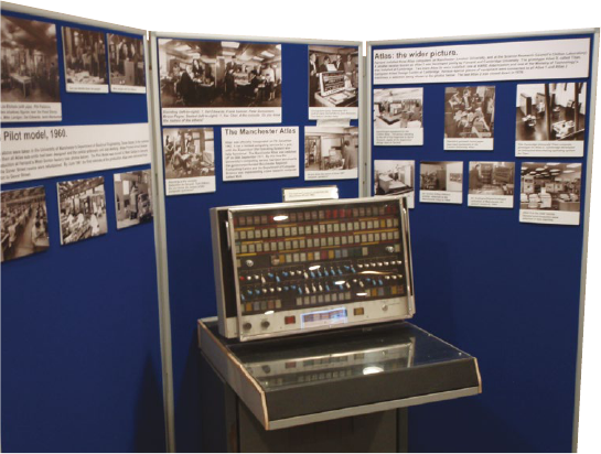
Operang Systems Foundaons with Linux on the Raspberry Pi
128
Each data item has an address (its index in the conceptual array) and a value (the bits stored at that
address). Low-level machine instrucons allow us to access data at byte, word, or mul-word
granularity, where a word might be 32 or 64 bits, depending on the plaorm conguraon. The Arm
instrucon set is a classic load/store architecture, with explicit instrucons to read from (i.e., LDR)
and write to (i.e., STR) memory.
6.3.2 Virtual addressing
In common with all modern high-level OSs, Linux uses virtual addressing. This is dierent from
microcontrollers like typical Arduino and Mbed devices, which perform direct physical addressing.
In Linux, each process has its own virtual address space, with virtual addresses (also known as logical
addresses) mapped onto physical addresses, conceptually as a one-to-one mapping.
Historically the Atlas computer, built at the University of Manchester in the 1960s, was the rst
machine to implement virtual memory. Figure 6.4 shows the original installaon. The system was
designed to map disparate memory technology onto a single address space, with address translaon
support in dedicated hardware.
Figure 6.4: The Atlas machine, designed at the University of Manchester, was the rst system to feature virtual memory. Photo by Jim Garside.
Several key benets are enabled by virtual memory.
Process isolaon: It is impossible to trash another process’ memory if the currently execung process
is unable to address that memory directly. Accessing ‘wild’ pointers may cause a segmentaon fault,
but this will only impact the currently execung program, rather than the enre system.
Code relocaon: Binary object les are generally loaded at the same virtual address, which is
straighorward for linking and loading tools. This can ensure locality in the virtual address space,
minimizing problems with memory fragmentaon.
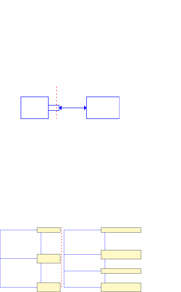
129
Hardware abstracon: The virtual address space provides a uniform, hardware-independent view of
memory, despite physical memory resources changing when we install more RAM or modify a hosted
VM conguraon.
Virtual addressing requires direct, integrated hardware support in the form of a memory management
unit (MMU). The MMU interposes between the processor and the memory, to translate virtual
addresses (in the processor domain) to physical addresses (in the memory domain). This translaon
process is known as hardware-assisted dynamic address relocaon and is supported by all modern
processor families. The rened Von Neumann architecture in Figure 6.5 gives a schemac overview
of the MMU’s interposing role.
Figure 6.5: Rened Von Neumann architecture showing the Memory Management Unit (MMU).
When the OS boots up, the processor starts in a physical addressing conguraon with the MMU
turned o. The early stages of the kernel boot sequence inialize basic data structures for virtual
memory management; then the MMU is turned on. For the Linux boot sequence on Arm, this happens
in the ___turn_mmu_on procedure in arch/arm/kernel/head.S.
6.3.3 Paging
The Linux virtual address space layout (for 32- and 64-bit Arm architectures) is shown in Figure
6.6. The split between user-space and kernel-space is either 3:1 or 2:2, for the 4GB address space.
The default Raspberry Pi Linux kernel 32-bit conguraon species CONFIG_VMSPLIT_2G=y which
means a 2:2 split. The 64-bit address boundary literals in Figure 6.6 assume eecve 39-bit virtual
addresses; several other variants are possible.
Figure 6.6: Linux virtual address space map for 32- and 64-bit architectures, lower addresses at the top.
i
i
“chapter” — 2019/8/13 — 18:08 — page 5 — #5
i
i
i
i
i
i
Processor MMU
Memory
Bus
virtual addresses physical addresses
i
i
“chapter” — 2019/8/13 — 18:08 — page 6 — #6
i
i
i
i
i
i
user space
kernel mem
0
0x80000000
2GB
0xFFFFFFFF
4GB
user space
unused
kernel mem
0
0x0000008000000000
512GB
0xFFFFFF8000000000
0xFFFFFFFFFFFFFFFF
16EB
32-bit addressing 64-bit addressing
Chapter 6 | Memory management
Operang Systems Foundaons with Linux on the Raspberry Pi
130
The parcular mechanism chosen to implement virtual addressing in Linux is paging, which supports
ne-grained resource allocaon and management of physical memory. In a paged memory scheme,
physical memory is divided into xed-size frames. Virtual memory is similarly divided into xed-sized
pages, where a single page has the same size as a single frame. This allows us to set up a mapping
from pages to frames. The typical size of a single page in Linux is 4KB on a 32-bit Arm plaorm.
Try getconf PAGESIZE on your terminal to nd your system’s congured page size in bytes.
The default page size is small enough to minimize fragmentaon but large enough to avoid excessive
overhead for per-page metadata. A page is the minimum granularity of memory that can be allocated
to a user process. Larger pages are supported navely on Arm. For instance, 64KB pages and mul-
MB ‘huge’ pages are possible. The advantage of larger pages is that fewer virtual to physical address
translaon mappings need to be stored. The main disadvantage comes from internal fragmentaon,
where a process is unable to use such a large amount of conguous space eecvely. Eecvely,
internal fragmentaon means there is free memory which belongs to one process and cannot be
assigned to another process. Generally, huge pages are appropriate for database systems and similar
specialized data-intensive applicaon workloads.
The next secon examines the underlying mechanisms required to translate page-based virtual
addresses into physical addresses.
6.4 Page tables
During normal process execuon, the processors and caches operate enrely in terms of virtual
addresses. As outlined above, the MMU intercepts all memory requests and translates virtual
addresses into physical addresses.
The translaon process relies on a mapping table, known as a page table which is stored in memory,
see Secons 6.4.1 and 6.4.2. Dedicated MMU base registers are available to point to page tables for
rapid access. An MMU cache of frequently used address mappings is maintained in the translaon
look-aside buer, see Secon 6.4.4.
Generally, the address translaon is performed by the MMU hardware, transparently from the process
or OS point of view. However, the OS is involved when a translaon does not succeed—this causes
a page fault, see Secon 6.5.2. Further, when a process begins execuon, the OS needs to set up the
inial page table and subsequently maintain it as the virtual address space evolves.
Somemes OS needs to operate on physical addresses directly, perhaps for device driver interacons.
There are macros to convert between virtual and physical addresses, e.g., virt_to_phys(), but
these only work for memory buers allocated by the kernel with the kmalloc roune.
6.4.1 Page table structure
The page table is an in-memory data structure that translates from virtual to physical addresses.
The translaon happens automacally through the MMU hardware, which is directly supported by
the processor. The MMU will automacally read the translaon tables when necessary; this process
is known as a page table walk. The OS simply has to maintain up-to-date mapping informaon in each
process’s page table, and refresh the page table base register each me a dierent process is execung.
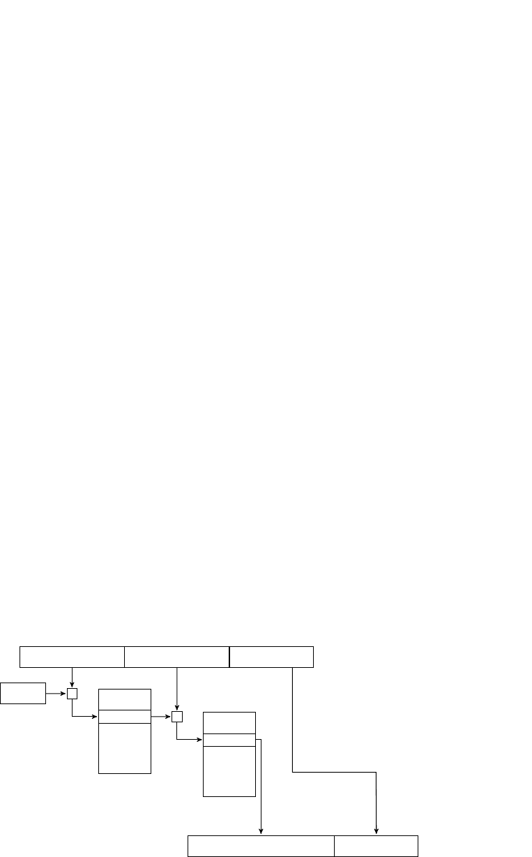
131
The simplest possible structure is a single-level page table. For each page in the virtual address space,
there is an entry in the table which contains a value corresponding to the appropriate physical address.
This wastes space—a typical 32-bit 4GB address space, divided into disnct 4K pages, will need
a single-level page table to contain 1M entries. Each entry consists of an address, say 4B, along with
some metadata bits. However, most processes do not make use of their enre virtual address space,
so many page table entries would remain unused.
This movates the design of a hierarchical page table. Before we get into specic details for Linux on Arm,
let’s consider an idealized two-level page table. A typical 32-bit virtual address is divided into three parts:
1. A 10-bit rst-level page table index.
2. A 10-bit second-level page table index.
3. A 12-bit page oset.
Given that pages are 4KB, this is a convenient subdivision. The 10 bits enable us to address 1024 32-
bit word entries. Each entry can contain a single address. This means each sub-table of the page table
can t into a single page.
For unused regions of the address space, the OS can invalidate corresponding entries in the rst-level
page table, as a consequence of which, we do not need second-level page tables for these address
ranges. This is the main space-saving for hierarchical page tables since each invalid rst-level page table
entry corresponds to 1024 invalid second-level page table entries—potenally saving up to 4MB of
second-level page table space.
Figure 6.7 gives a schemac overview of a single virtual address translaon, as handled by the MMU,
using the two-level page table outlined above. Note the consecuve pair of table indexing operaons,
based on the P1 and P2 bitelds in the virtual address. The entry in the second-level page table
contains the physical frame number, which is concatenated bitwise with the page oset to generate
the actual physical address. There are spare bits in the 32-bit page table entry since the frame number
will only occupy 20 bits. These remaining (low-order) bits can be used for page metadata such as
access permissions, see Secon 6.4.3.
Figure 6.7: Virtual address translaon via a two-level page table.
i
i
“chapter” — 2019/8/13 — 18:08 — page 7 — #7
i
i
i
i
i
i
P1 index P2 index
page offset
+
base register
first-level
table
entry
+
second-level
table
entry
page offset
frame number
Chapter 6 | Memory management
Operang Systems Foundaons with Linux on the Raspberry Pi
132
An n-level hierarchical page table will impose an overhead of n (page table) memory references for
each ‘actual’ memory reference. There are techniques to migate this overhead; for instance, see
Secon 6.4.4.
6.4.2 Linux page tables on Arm
This secon explores how the Linux model for page tables is realized on the Arm architecture.
First, we examine the generic Linux page table architecture; then we review the plaorm-specic
opmizaons that are enabled for the Raspberry Pi.
Linux supports a mul-level hierarchical page table. Since kernel version 4.14, page tables can have up
to ve levels.
1. PGD, page global directory: one per process, with a base pointer stored in an MMU register,
and in the process state context at current->mm.pgd.
2. P4D, fourth level directory: only applicable to 5-level page tables, currently not supported on Arm.
3. PUD, page upper directory: applicable to 4- and 5-level page tables, currently supported on
AArch64.
4. PMD, page middle directory: intermediate level table.
5. PTE, page table entry: a leaf of the page table, containing mulple pages to frame translaons.
With some plaorms, fewer hardware page table levels are available than the Linux kernel supports.
For instance, the default 32-bit Raspberry Pi Linux kernel conguraon uses a two-level page table,
as documented in arch/arm/asm/pgtable-2level.h. The PMD is dened to have a nominal size
of single entry; it folds back directly onto the page global directory (PGD), which is opmized away at
compile me. This unit-sized intermediate page table ‘trick’ is also applied to other architectures and
conguraons.
The two-level page table structure maps neatly onto the Arm MMU paging hardware in the Raspberry
Pi Broadcom SoC, which has a two-level page table where the rst level contains 4096 entries (i.e.,
4 consecuve pages) and each of the second level tables has 256 entries. Each entry is a 32-bit word.
However, because the Arm MMU hardware does not provide a suciently rich set of page metadata
for the Linux memory manager, the metadata bits for each page have to be managed in soware, via
page faults and soware xups. For instance, Linux requires a ‘young’ bit for each page. This bit tracks
whether the page has been accessed recently, which is useful for page replacement policies. The
‘young’ bit is not supported navely on Arm.
Linux sees the abstracon of 2048 64-bit entries in the PGD, dened in the pgtable-2level.h
with #denePTRS_PER_PGD2048. Each 64-bit PGD composite entry breaks down into two 32-bit
pointers to consecuve second-level blocks. Since the Arm MMU supports 256 entries in a second-
level page table block, then there are 512 entries in two consecuve blocks. Thus Linux sees the

133
abstracon of 512 32-bit entries in a logical PTE. This is dened in the pgtable-2level.h le with
#denePTRS_PER_PTE512.
These PTE blocks only occupy half a 4KB page. The other half is occupied by arrays of Linux per-page
metadata, which is not supported navely by the Arm MMU. Eecvely, the Linux PTE metadata
shadows the Arm hardware-supported metadata and is maintained by the OS using a page fault
and xup mechanism. The relevant code is in set_pte_ext, which is generally implemented as an
assembler intrinsic roune, for eciency reasons. For instance, check out the assembler roune
cpu_v7_set_pte_ext in le arch/arm/mm/proc-v7-2level.S. The hardware page metadata
word is generally 2048 bytes ahead of the corresponding Linux shadow metadata. To nd this, execute
the command:
grep -4, 2048 *.S
Bash
in the linux/arch/arm/mm/ directory. Secon 6.4.3 outlines the Linux metadata that the OS
maintains for each page.
Eecvely, two dierent page table mechanisms are superimposed seamlessly onto the one-page
table data structure, for both the Arm MMU and the Linux virtual memory manager. Figure 6.8 shows
this page table organizaon as a schemac diagram.
Figure 6.8: Linux page table organizaon ts into the Arm hardware-supported two-level paging structure, with Linux page metadata bits shadowing
hardware metadata at a distance of half a page (2048 bytes).
There are several more complex variants on this virtual addressing scheme. For instance:
1MB secons are conguous areas of physical memory that can be translated directly from a single
PGD entry. This enables more rapid virtual address translaon.
Large Physical Address Extension (LPAE) is a scheme that enables 32-bit virtual addresses to be
mapped onto 40-bit physical addresses. This permits 1TB of physical memory to be used on 32-bit
Arm plaorms.
i
i
“chapter” — 2019/8/13 — 18:08 — page 8 — #8
i
i
i
i
i
i
ptr1
ptr2
256 h/w entries
256 h/w entries
256 Linux flagsets
256 Linux flagsets
2 Arm top-level
entries (8 bytes)
4 Arm 2nd-level blocks
(4K, 1 page)
Chapter 6 | Memory management

Operang Systems Foundaons with Linux on the Raspberry Pi
134
6.4.3 Page metadata
To avoid confusion, note that a ‘page table entry’ may refer to one of two dierent concepts:
1. A Linux PTE, which is a leaf in the page table, containing 512 mappings from virtual to physical
addresses.
2. A single mapping from a virtual to a physical address, along with corresponding metadata.
Throughout this chapter, when we mean (1), we will refer to it as a ‘Linux PTE’ specically.
As well as recording the page frame number, to perform the mapping from a virtual to a physical
address, a page table entry also stores appropriate metadata about the page. This includes informaon
related to memory protecon, sharing, and caching. Individual bits in the page table entry are
reserved for specic informaon, so the OS can nd aributes of pages with simple bitmask and shi
operaons.
Linux devotes a number of PTE bits to metadata. A typical layout is below, for the Raspberry Pi two-
level pagetable (consult le arch/arm/include/asm/pgtable-2level.h for details).
If a process aempts to make an illegal memory access (e.g., if it tries to execute code in a non-
executable page or to read data from an invalid page), then a page fault event occurs and the system
traps to a page fault handler, see Secon 6.5.2.
From a user perspecve, the simplest way to see memory metadata is to look at the /proc/PID/
maps le for a process. Although the informaon is not presented at page level, it is shown at the level
of segments, which are conguous page sequences in the virtual address space. For each segment, the
permissions are listed: these might include read (r), write (w), and execute (x). A further column shows
whether the memory is private (p) to this process or shared (s) between mulple processes.
Table 6.1: Metadata associated with each page table entry in Linux.
Macro Descripon Bit posion
L_PTE_VALID
Is this page resident in physical memory, or has it been swapped out? 0
L_PTE_YOUNG
Has data in this page been accessed recently? 1
—
4 bits associated with cache residency 2–5
L_PTE_DIRTY
Has data in this page been wrien, so the page needs to be ushed to disk? 6
L_PTE_RDONLY
Does this page contain read-only data? 7
L_PTE_USER
Can this page be accessed by user-mode processes? 8
L_PTE_XN
Does this page not contain executable code? (protecon for buer overow aaches) 9
L_PTE_SHARED
Is this page shared between mulple process address spaces? 10
L_PTE_NONE
Is this page protected from unprivileged access? 11
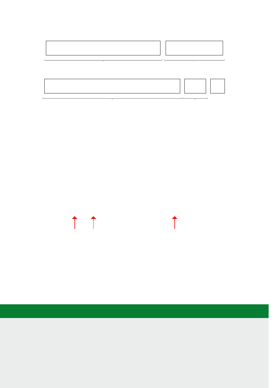
135
Figure 6.9: Bitmap paerns for page table entries, for a resident page to frame translaon (above) and for a non-resident (swapped out) page (below).
Figure 6.10 shows an example of this memory mapping data for a single Linux process.
Figure 6.10: Extract from a process memory mapping reported in /proc/PID/maps.
The binary le /proc/PID/pagemap records actual mapping data. Access to this le requires root
privileges, otherwise reads return zero values or cause permission errors. The pagemap le has
a 64-bit value for each page. The low 54 bits of this value correspond to the physical address or swap
locaon of that page. Higher bits are used for page metadata. The Python code below performs
a single virtual to physical address translaon using this map.
Lisng 6.4.1: Reading from the /proc pagemap le Python
1 import sys
2
3 pid = int(sys.argv[1], 10) # specify as decimal
4 vaddr = int(sys.argv[2], 16) # specify as hex
5
6 PAGESIZE=4096 # 4K pages
7 ENTRYSIZE=8
8
9 with open(("/proc/%d/pagemap" % pid), "rb") as f:
10 f.seek((vaddr/PAGESIZE) * ENTRYSIZE)
11 x = 0
i
i
“chapter” — 2019/8/13 — 18:08 — page 10 — #10
i
i
i
i
i
i
31 12
page index
11 0
metadata
31 9
swap entry
8 3
swap type
000
2 0
i
i
“chapter” — 2019/8/13 — 18:08 — page 11 — #11
i
i
i
i
i
i
pi@raspberrypi:/home/pi $ cat /proc/23655/maps
00010000-00011000 r-xp 00000000 b3:02 42164 /home/pi/.../a.out
00020000-00021000 rw-p 00000000 b3:02 42164 /home/pi/.../a.out
76e67000-76f92000 r-xp 00000000 b3:02 1941 /lib/arm-.../libc-2.19.so
76f92000-76fa2000 ---p 0012b000 b3:02 1941 /lib/arm-.../libc-2.19.so
76fa2000-76fa4000 r--p 0012b000 b3:02 1941 /lib/arm-.../libc-2.19.so
76fa4000-76fa5000 rw-p 0012d000 b3:02 1941 /lib/arm-.../libc-2.19.so
76fa5000-76fa8000 rw-p 00000000 00:00 0
76fa8000-76fad000 r-xp 00000000 b3:02 10133 /usr/lib/.../libarmmem.so
76fad000-76fbc000 ---p 00005000 b3:02 10133 /usr/lib/.../libarmmem.so
76fbc000-76fbd000 rw-p 00004000 b3:02 10133 /usr/lib/.../libarmmem.so
76fbd000-76fdd000 r-xp 00000000 b3:02 1906 /lib/arm-.../ld-2.19.so
address range
access permissions
mapped file
Chapter 6 | Memory management
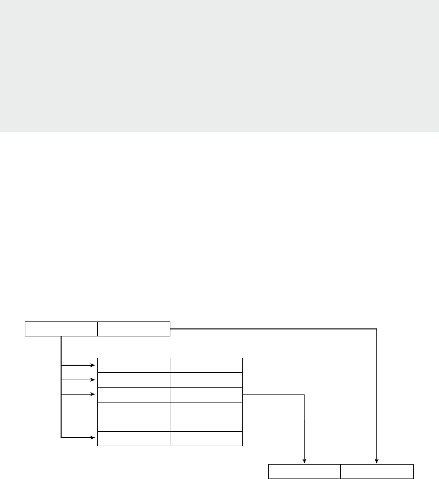
Operang Systems Foundaons with Linux on the Raspberry Pi
136
12 for i in range(ENTRYSIZE):
13 x = (ord(f.read(1))<<(8*i)) + x # little endian
14
15 # interpret entry
16 present = (x>>63) & 1
17 swapped = (x>>62) & 1
18 le_page=(x>>61)&1
19 soft_dirty =(x>>54) & 1
20
21 paddr = x & ((1<<32)-1)
22
23 print ("virtual address %x maps to **%d%d%d%d** %x" %
24 (vaddr,present,swapped,le_page,soft_dirty,(paddr*PAGESIZE)))
6.4.4 Faster translaon
Since every access to main memory requires an address translaon, it is helpful to cache frequently
used translaons to reduce overall access latency. The micro-architectural component that supports
this address translaon caching is known as a translaon look-aside buer (TLB). This is a fully
associave cache that stores a small set of virtual to physical (i.e., page to frame number) mappings.
Accessing data in the TLB is much quicker than a page table lookup; a TLB access may take only
a single cycle, at least one order of magnitude faster than a full page table walk. Figure 6.11 shows
how a TLB works. When a virtual address needs to be translated, the TLB looks up all its (page,
frame) entries in parallel. If any page tag matches then we have a TLB hit. The translaon succeeds
with minimal overhead. On the other hand, if no entry tag matches then we have a TLB miss, and an
expensive page table lookup is necessary.
Figure 6.11 Fast virtual address lookup with a translaon look-aside buer.
Eecve use of the TLB depends on the same memory access behavior as for standard caches,
i.e., spaal and temporal locality of data accesses. If we can maximize TLB hits, most memory
addresses will be translated without needing to access the page table in main memory. Thus, in the
common case, the performance will be the same as for direct physical addressing; the TLB minimizes
translaon overhead.
i
i
“chapter” — 2019/8/13 — 18:08 — page 12 — #12
i
i
i
i
i
i
page number
page offset
p
o
p
1
p
2
p
n
...
f
o
f
1
f
2
f
n
...
frame number
frame offset
TLB hit
virtual address
physical address
fully associative cache

137
The Arm Cortex A53 processor in the Raspberry Pi 3 features a two-level TLB. Each core has a micro-
TLB, with 10 entries for instrucon address lookups, and a further 10 for data address lookups. This
corresponds to the Harvard architecture of the L1 cache. The main TLB is a 512 entry 4-way set
associave cache. Each entry is tagged with a process-specic address space idener (ASID) or is
global for all applicaon spaces. The hardware automacally populates and maintains the state of
the TLB; although, if the OS modies an address translaon that is cached in the TLB, it is then the
responsibility of the OS to invalidate this stale TLB entry.
Since the TLB caches virtual addresses, its data must be ushed when the virtual address space
mapping changes, perhaps at an OS context switch. The Arm system coprocessor has a TLB
Operaons Register c8, which supports TLB entry invalidaon. There are dierent opons for how
much to invalidate since a TLB ush is parcularly expensive in terms of its impact on performance.
For instance, it is not necessary to ush kernel addresses, since the kernel address space is common
across all processes in the system. Each process may be associated with a disnct ASID, and only
entries linked with the relevant ASID need to be invalidated on a context switch.
6.4.5 Architectural details
In the Arm architecture model, the system control coprocessor CP15 is responsible for the
conguraon of memory management. Translaon table base registers (TTBRs) in this unit are
congured to point to process-specic page tables by the OS, on a context switch. These registers
are only accessible in privileged mode.
To read TTBR0 into general purpose register r0, we use the instrucon:
MRC p15, 0, r0, c2, c0, 0
where p15 is the coprocessor, and c0 and c2 are coprocessor-specic registers. The dual MCR
instrucon writes from r0 into TTBR0, to update the page table base pointer.
Generally, Arm uses a one-page table base register for process-specic addresses (TTBR0) and
devotes the other for OS kernel addresses (TTBR1). The page table control register TTBCR determines
which page table base register is used for hardware page table walks; TTBCR is set when we vector
into the kernel.
When the OS performs a context switch, it updates the process page table root pointer, PGD, to
switch page tables. Since the on-chip caches are indexed using virtual addresses, it may be necessary
to ush the cache on a context switch as well. Since this is a high-overhead operaon, there are
various techniques to avoid cache ush on context switch. These opmizaons may require more
complex cache hardware (e.g., ASIDs per cache line) or more intricate OS memory management
(e.g., avoid overlaps in virtual address space ranges between concurrent processes).
Chapter 6 | Memory management

Operang Systems Foundaons with Linux on the Raspberry Pi
138
6.5 Managing memory over-commitment
Since a process virtual address space may be much larger than the available physical memory, it is
possible to allocate more memory than the system contains. This supports the abstracon that the
system appears to have more memory than is physically installed. Recall that each process has
a separate virtual address space (VAS); all VASs are mapped onto a single physical address space.
This memory over-commitment is managed by the OS.
6.5.1 Swapping
When the system has more pages allocated than there are frames available in physical memory, the
OS has to swap pages out of RAM and into the backing store. The Linux swap facility handles this
overow of pages. Swapping in Linux is oen referred to as paging in other OS vocabularies.
Swap space is persistent storage, generally orders of magnitude slower than RAM. Typical swap space
is a le system paron or a large le on the root le system. Check out cat /proc/swaps to inspect
swap storage facilies on your Raspberry Pi Linux device. The Raspian default swap facility is a single
100MB le in /var/swap.
sudo hexdump -C /var/swap | less
Bash
Examine to see what is stored in the swap space currently, although much of this data may be stale
copies of old pages. Look for the SWAPSPACE2 magic header near the start of the le. In general,
the swap le is divided up into page-sized slots. Note that swapping is not parcularly common on
Raspberry Pi since access latency to SD card storage is parcularly high and frequent access can cause
device corrupon.
In a process page table, individual entries may be marked as swapped out. The pte_present()
macro checks whether a page is resident in memory or swapped out to disk. The biteld layout of the
page table entry for a swapped out page is shown in Figure 6.9, with disnct elds for the swap device
number and the device-specic index.
A process may execute when some of its pages are not resident in memory. However, the OS needs
to handle the situaon when the process tries to execute a memory access from a swapped out (non-
resident) page. The next secon describes this OS support for page faults.
6.5.2 Handling page faults
A page fault event is a processor excepon, which must be handled by an OS-installed excepon
handler. In Linux, the page fault handler is do_page_fault(), dened in arch/arm/mm/fault.c,
which calls out to non-architecture-specic rounes in mm/memory.c.
Figure 6.12 depicts a simplied ow graph for the page fault handling code. Inially, the
handler checks whether this page is a sensible page for the process to be accessing, as opposed to
a ‘wild’ access outside the process’ mapped address space. Then there is a permissions check of the
page table entry to determine whether the process is allowed to perform the requested memory
operaon (read, write, or execute). If either check fails, then there is a segmentaon fault. If the checks
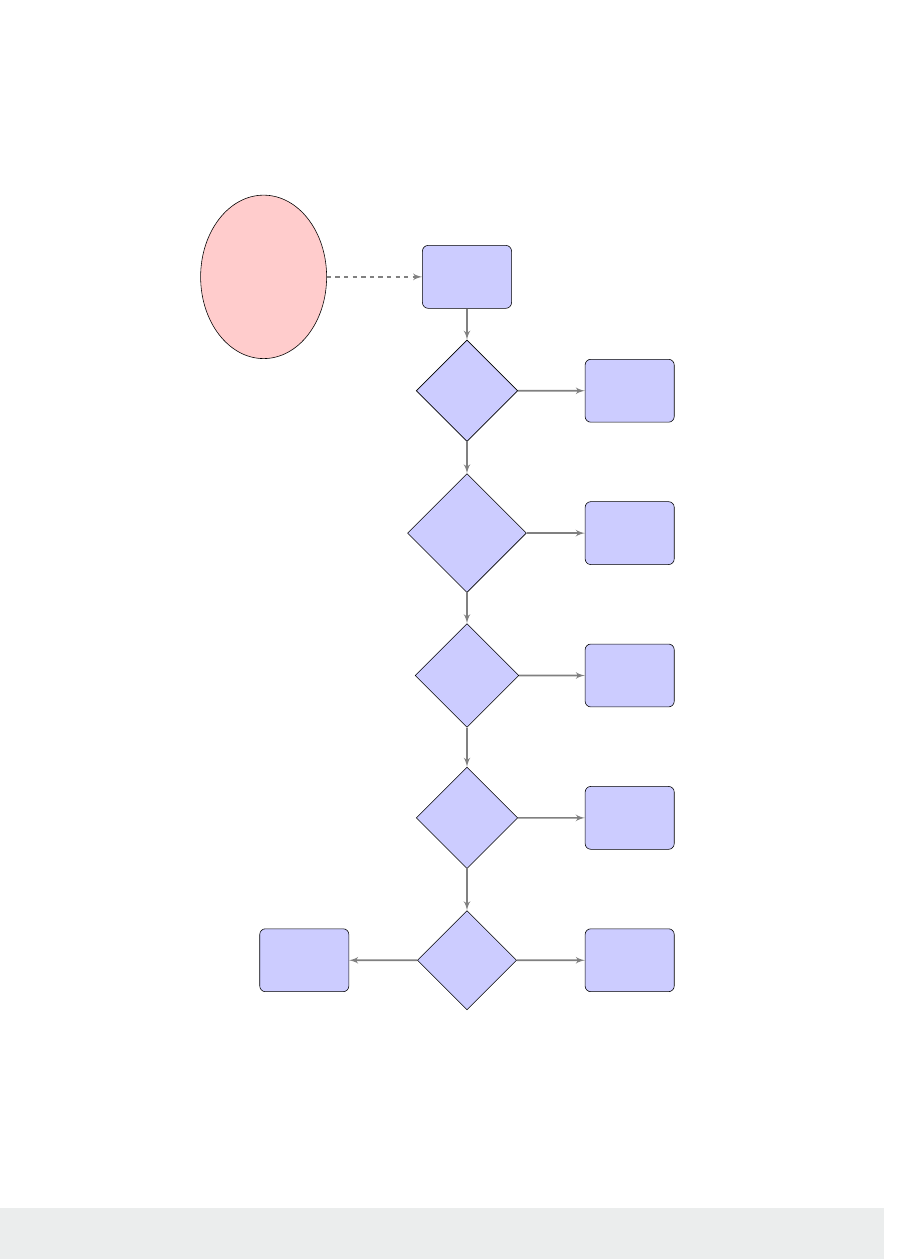
139
pass, then the page fault handler will take appropriate remedial acon, swapping in a swapped out page,
reading in data from a le, performing a copy on write operaon, or allocang a fresh frame for a new page.
Figure 6.12: Flow chart for Linux page fault handling code.
Once the page fault has been handled, the OS restarts the faulng process at the instrucon that
originally caused the excepon, and user-mode execuon resumes, subject to process scheduling.
Suppose you have just launched a process with PID 6903, you can inspect the actual page faults
incurred by this process with the command:
ps-omin_t,maj_t,cmd,args6903
Bash
i
i
“chapter” — 2019/8/13 — 18:08 — page 13 — #13
i
i
i
i
i
i
page fault
handler
page fault
exception
for address
x with
access
mode M
is x invalid
address?
signal a
segfault
is M
forbidden
at x?
signal a
segfault
is data for
x in swap?
swap in
page data
is data for
x in a file?
read in
file data
is page at x
resident?
do copy
on write
alloc fresh
empty page
trap
no
no
no
yes
no
yes
yes
yes
yes
no
Chapter 6 | Memory management

Operang Systems Foundaons with Linux on the Raspberry Pi
140
Running the command without a PID integer argument lists stascs for all the user’s processes. To
run a program and get a total count for its page faults, use the /usr/bin/time command. (This may
require you to install the time package with sudo apt-get install time. Note you need the
full path, since time is also a bash built-in command). Now try /usr/bin/time ls and see how the
output reports the number of page faults.
Note that Linux disnguishes between minor faults — when a page is already resident, but not mapped
in this process’ VAS (e.g., code shared between mulple processes), and major faults — when the OS
has to access the persistent store and read in data from a le.
As an example, consider the C code below. It creates a mul-page array and accesses a single byte
in each page. Because of demand paging, the pages are only mapped into the process’ VAS when rst
accessed. As the program is executed with larger sized arrays (use the command line parameter to
increase the size) the number of minor page faults increases. Try running it with an argument of 64000
(256MB sized array). Note if there is not enough memory, then the program will terminate.
Lisng 6.5.1: Program that induces minor page faults C
1 #include <stdlib.h>
2
3 /* assume 4KB page size */
4 #dene PAGES 1024*4
5
6 int main(int argc, char **argv) {
7 char *p = 0;
8 int i = 0, j = 0;
9 /* n is number of pages */
10 int n = 100;
11 if (argc == 2) {
12 n = atoi(argv[1]);
13 }
14 p = (char *)malloc(PAGES*n);
15 for (i=0; i<PAGES; i++) {
16 for (j=0; j<PAGES*(n-1); j+=PAGES) {
17 p[(i+j)] = 42;
18 }
19 }
20 return 0;
21 }
Now consider a similar program, but one that uses memory-mapped les, so the OS has to fetch the
data from the backing store. Grab a text le, e.g., with:
curl-oalice.txthttp://www.gutenberg.org/les/11/11-0.txt
Bash
and then compile the code shown below.

141
Lisng 6.5.2: Program that induces major page faults C
1 #include <assert.h>
2 #include <fcntl.h>
3 #include <stdio.h>
4 #include <sys/mman.h>
5 #include <sys/stat.h>
6 #include <unistd.h>
7
8 size_t get_size(const char*lename){
9 struct stat st;
10 stat(lename,&st);
11 return st.st_size;
12 }
13
14 int main(int argc, char** argv) {
15 int i, total = 0;
16 size_tlesize=get_size(argv[1]);
17 int fd = open(argv[1], O_RDONLY, 0);
18 char *data;
19 assert(fd != -1);
20 posix_fadvise(fd,0,lesize,POSIX_FADV_DONTNEED);
21 data = mmap(NULL,lesize,PROT_READ,MAP_PRIVATE|
22 MAP_NONBLOCK, fd, 0);
23 assert(data != MAP_FAILED);
24 for(i=0;i<lesize;i+=1024)
25 total += data[i];
26 printf("total = %d\n", total);
27 intrc=munmap(data,lesize);
28 assert(rc==0);
29 close(fd);
30 }
The rst me you run this program with:
/usr/bin/time -v ./a.out alice.txt 2>&1 | grep Major
Bash
noce there is at least one major fault as the le is read into memory. However, if you run it
immediately again, for a second me, there will be no major faults; the le data is already cached in
memory, so the program only causes minor faults.
6.5.3 Working set size
The working set for a process measures the number of pages that must be resident for that process to
make useful progress, i.e., to avoid constant swapping.
There are various les that track per-process memory consumpon. For instance, for a process with
id PID, the le /proc/PID/statm reports page-level memory usage. The rst column shows the
vmsize (the number of pages allocated in the virtual address space) , and the second column shows
the resident set size (the number of pages resident in physical memory for this process). The following
inequality always holds: rss < vmsize. The le /proc/PID/status shows the same informaon in
a more readable format.
Chapter 6 | Memory management

Operang Systems Foundaons with Linux on the Raspberry Pi
142
For a process to execute eecvely, the RSS should be at least as large as the working set size (WSS).
Linux does not measure WSS directly; however, various third-party scripts are available to esmate
process WSS, e.g., consult hp://www.brendangregg.com/wss.html
6.5.4 In-memory caches
Physical memory frames that are not being used to store process pages could be used eecvely by
the OS for other purposes, such as caching data. Linux features several kinds of in-memory caches
that use these free frames.
The le system page cache stores page-sized chunks of les in memory, aer they are rst touched.
The OS reads ahead, to load porons of the le into memory in ancipaon of future accesses.
The fadvise funcon allows the process to specify how the le will be accessed. The page cache
is the reason why second and subsequent accesses to a le generally take much less me than the
inial access.
The swap cache keeps track of which physical frames have been wrien out to a swap le. This is
highly useful for pages shared between mulple processes, for example. Once a page has been wrien
out to the swap le, then the next me the page is swapped in, the data remains in the swap le slot.
If this page is not modied aer regaining memory residence, and then at some later stage it needs to
be swapped out again, we can avoid the writeback if it has not been modied since the last swap in.
The swap le records where the page lives in swap, so we can record this in the relevant page table
entry. On the other hand, if the page is modied in memory, then its swap cache entry is expunged
because the page becomes dirty and must be wrien back. This swap cache feature may save
unnecessary swap le writebacks.
The buer cache is used to opmize access to block devices (see later chapter on I/O). Since read and
write operaons are expensive for slow block devices, the buer cache interposes these accesses to
reduce I/O latency. For instance, individual writes from a collecon of processes could be batched up
for a block device. A buer cache will record blocks of data that have been read from or wrien to
a block device.
We can use commands like free -h or vmstat -S m to inspect how the Raspberry Pi physical
RAM is allocated between process pages, OS buers, page cache, etc. Ideally, all unused frames in
a system would be occupied by buers and caches, since this is preferable to underulizing physical
RAM. Then the caches are shrunk when the process page requirements increase as more processes
are admied.
6.5.5 Page replacement policies
The kernel swap daemon is a background process that commences running aer kernel inializaon.
ps -eo | grep kswapd
Bash
Invoke to see this daemon running on your Pi. The responsibility of kswapd is to swap out pages that
are not currently needed. This serves to maintain a set of free frames that are available for newly
allocated or swapped in pages.

143
Some pages are obvious candidates for swapping out; these are clean pages whose data is already in
the backing store, e.g., executable code, other memory-mapped les, or pages in the swap cache. Such
pages can be discarded without copying any data since the data is already stored elsewhere. On the
other hand, dirty pages have been updated since they were read in from backing store; other pages
(e.g., anonymous process pages) may never have been wrien out to the backing store. Such pages
must have their data transferred to persistent storage before they can be swapped out.
It is not ecient to swap out pages if their data may be required again in the near future since the
swap out operaon will be followed swily by a swap in of the same data.
Bélády’s opmal page replacement policy is a theorecal oracle that looks into the future, to select
a candidate page for replacement that will not be used again, or will only be used further in the future
than any other page currently resident. Since this abstracon is not implementable, Linux assumes
that, if a page has not been used in the recent past, then it is unlikely to be used again in the near
future. This is the principle of temporal locality.
Two memory manager mechanisms are used to keep track of page usage over me:
1. Each page has an associated metadata bit that may be set when the page is accessed.
2. Pages may be stored in a doubly-linked list that approximates least-recently-used (LRU) order.
Pages grow older as they are not accessed over me; old pages are ideal candidates for swapping out.
Below we review several page replacement policies.
Random
The simplest page replacement algorithm does not take page age or usage into account. It simply
selects a random vicm page to be swapped out immediately, to make space for a new page.
Not recently used
A page is not recently used (NRU) if its access metadata bit is unset. Such a page is a good candidate
for replacement. The NRU algorithm might work as follows:
1. A page p is randomly selected as a candidate.
2. If p access bit is set, go back to (1).
3. Assert p access bit is unset, and select p for replacement.
There is no guarantee of terminaon with NRU, since all pages may have access bits set. We assume
the OS will periodically unset all bits.
Clock
The clock algorithm keeps a circular list of pages. There is a conceptual ‘hand’ that points to the next
candidate page for replacement, see Figure 6.13. When a page replacement needs to take place, the
Chapter 6 | Memory management
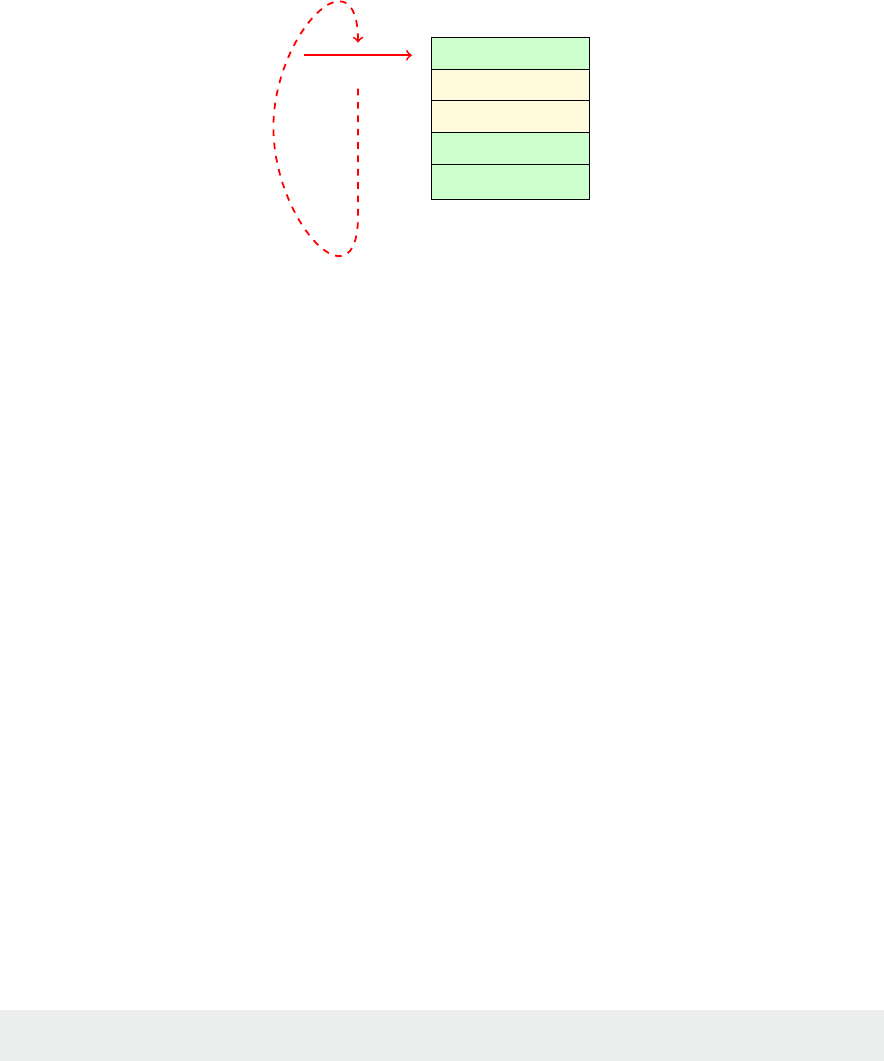
Operang Systems Foundaons with Linux on the Raspberry Pi
144
clock algorithm inspects the current candidate—if its access bit is set, then the access bit is unset and
the clock hand advances to the next page. The rst page with an unset access bit is selected as the
vicm to be swapped out. This is a ‘second chance’ algorithm.
Figure 6.13: Clock page replacement algorithm.
Least recently used
A genuine least recently used (LRU) scheme either upgrades the single access biteld to a longer, last
access mestamp eld for each page, or shues pages in a doubly-linked list to sort them in order of
access me. The vicm page is then easily selected as the page with the oldest mestamp, or the page
at the tail of the list respecvely. Both of these techniques have signicant management overhead.
The Linux memory manager actually implements a variant of the LRU page replacement scheme.
Pages allocated to processes are added to the head of a global acve pages queue. When a page
needs to be evicted, the tail of this queue is examined. If the tail page has its access bit set, then it is
moved back to the head of the queue, and its access bit is unset. However, if the tail page does not
have its access bit set, then it is a candidate for replacement, and it is moved to the inacve pages
queue from where it may be swapped out.
The page replacement algorithm is implemented in funcon do_try_to_free_pages() in source
code le linux/mm/vmscan.c, but be aware that this is a complex piece of code to trace.
Tuning the system
Linux has a kernel parameter called swappiness, which controls how aggressively the kernel swaps
pages out to the backing store. The value should be an integer between 0 and 100 inclusive. Higher
values are more aggressive at swapping pages from less acve processes out of physical memory,
which improves le-system performance (cache).
Note that, on a Raspberry Pi device, the swappiness may set at a parcularly low value, since the swap le
or paron is on an SD card, which has high access latency and may fail with excessive write operaons.
Find your current system’s swappiness value with:
cat /proc/sys/vm/swappiness
Bash
i
i
“chapter” — 2019/8/13 — 18:08 — page 14 — #14
i
i
i
i
i
i
p
0
: accessed: 1
p
1
: accessed: 0
p
2
: accessed: 0
p
3
: accessed: 1
p
4
: accessed: 1
clock

145
On a desktop Linux installaon, the default value is generally 60. Try something like:
sudo sysctl -w vm.swappiness=100
Bash
and see whether this changes the performance of your system over me.
When the physical memory resource becomes chronically over-commied, acve pages must
be swapped out and swapped in again with increasing frequency. The whole system slows down
drascally since no process can make progress without incurring major page faults. All the system me
is spent servicing these page faults, so no useful work is achieved. The phenomenon is known
as thrashing, and it badly aects system performance.
6.5.6 Demand paging
Linux implements demand paging, which means physical memory is allocated to processes in a lazy,
or just-in-me, manner. A call to mmap only has an eect on the process page table; frames are not
allocated to the process directly. The process is only assigned physical memory resource when it really
needs it.
The Linux memory management subsystem records areas of virtual memory that are mapped in
the virtual address space, but for which the physical memory has not yet been allocated. (These are
zeroed-out entries in the page table.) This is the core mechanism that underlies demand paging: when
the process tries to access a memory locaon that is in this uninialized state, a page fault occurs, and
the physical memory is directly allocated. This corresponds to the boom le case (alloc fresh empty
page) in Figure 6.12.
The high-level layout of a process’ virtual address space is specied by the mm_struct data structure.
The process’ task_struct instance contains a eld that points to the relevant mm_struct. The
denion of mm_struct is in le include/linux/mm_types.h. It stores a linked list of vm_area_
struct instances, which model virtual memory areas (VMAs).
The list of VMAs encapsulates a set of non-overlapping, conguous blocks of memory. Each VMA
has a start- and end-address, which are aligned with page boundaries. The vm_area_struct, also
dened in include/linux/mm_types.h. has access permission ags, and prev and next pointers
for the linked list abstracon. Reading from /proc/PID/maps simply traces the linked list of VMAs
and prints out their metadata one-by-one, for instance, see Figure 6.10.
Each vm_area_struct also has a eld for a backing le, in case this VMA is a memory-mapped le.
If there is no le, this is an anonymous VMA which corresponds to an allocaon of physical memory.
When a page fault occurs for an address due to demand paging, the kernel looks up the relevant VMA
data via the mm_struct pointer. Each VMA has an embedded set of funcon pointers wrapped in
a vm_operations_struct. One of these entries points to a specic do_no_page funcon that
implements the appropriate demand paging behavior for this block of memory: the invoked acon
might be allocang a fresh physical frame for an anonymous VMA, or reading data from a le pointer
for a le-backed VMA.
Chapter 6 | Memory management

Operang Systems Foundaons with Linux on the Raspberry Pi
146
A process may use the madvise API call to provide hints to the kernel about when data is likely to
be needed, or what kind of access paern will be used for a parcular area of memory— sequenal
or random access, for instance.
6.5.7 Copy on write
When a child process is forked, it shares its parent’s memory (although logically it has a disnct,
isolated copy of the parent’s virtual address space). The child process virtual address space maps to the
same physical frames, unl either parent or child tries to write some data. At that stage, a fresh frame
is allocated dynamically for the wring process.
This copy on write mechanism is supported through duplicated page table entries between parent and
child processes, page protecon mechanisms, and sophiscated page fault handling, as outlined above.
Copy on write leads to ecient process forking; child page allocaon is deferred unl data write
operaons occur—pages are shared between parent and child unl their data diverges through write
operaons.
For a simple example of copy on write acvity, execute the source code below and check the measured
me overheads for the buer updates. Where the me is longest, then copy on write paging acvity is
taking place.
Lisng 6.5.3: Measuring overhead of copy on write acvity C
1 #include <errno.h>
2 #include <stdio.h>
3 #include <stdlib.h>
4 #include <time.h>
5 #include <unistd.h>
6
7 #dene PAGE_SIZE 4096
8 #dene NUM_PAGES 100000
9
10 void write_data(char*buer,int size) {
11 int i;
12 static char x = 0;
13 clock_t start, end;
14 start = clock();
15 for (i=0; i<size; i+=PAGE_SIZE)
16 buer[i]=x;
17 x++;
18 end = clock();
19 printf("time taken: %f seconds\n",
20 (double) (end-start) / CLOCKS_PER_SEC);
21 }
22
23 int main(int argc, char **argv) {
24 static charbuer[NUM_PAGES*PAGE_SIZE];
25 int res;
26
27 printf("1st test - expect high time - pages allocating\n");
28 write_data(buer,sizeofbuer);
29
30 switch(res = fork()) {
31 case -1:

147
32 fprintf(stderr,
33 "Unable to fork: %s(errno=%d)\n",
34 strerror(errno), errno);
35 exit(EXIT_FAILURE);
36 case 0: /* child */
37 printf("child[%d]: 2nd test - expect high time - copy on write\n", getpid());;
38 write_data(buer,sizeofbuer);
39 printf("child[%d]: 3rd test - expect low time - pages available\n", getpid());
40 write_data(buer,sizeofbuer);
41 exit(EXIT_SUCCESS);
42 default: /* parent */
43 printf("parent[%d]:waitingforchild[%d]tonish\n",
44 getpid(), res);
45 wait(NULL); /* child runs before parent */
46 printf("parent[%d]: 4th test - expect fairly low time - pages available"
47 "but not in processor cache\n", getpid());
48 write_data(buer,sizeofbuer);
49 exit(EXIT_SUCCESS);
50 }
51 }
Copy on write is a widely used technique. For instance, check out online informaon about ‘purely
funconal data structures’ to see how copy on write is used to make high-level algorithms and data
structures more ecient.
6.5.8 Out of memory killer
In the worst case, there is insucient physical memory available to support all running processes. The
kernel invokes a killer process (OOM-killer) at this stage, to idenfy a vicm process to be terminated,
freeing up physical memory resource. Heuriscs are used to idenfy memory hogging processes; look at
the integer value in /proc/PID/oom_score — higher numbers indicate more memory hogging processes.
It’s possible to invoke the OOM-killer manually. Run this memory-hogging Python script:
Lisng 6.5.4: A memory-hogging script Python
1 #!/usr/bin/python
2 import time
3 megabyte = (0,) * (1024 * 1024 / 8)
4 data = megabyte*400
5 time.sleep(60)
and then execute these bash commands:
Lisng 6.5.5: Trigger the OOM killer interacvely Bash
1 sudo chmod 777 /proc/sysrq-trigger # to allow us to trigger special events
2 echo "f" > /proc/sysrq-trigger # trigger OOM killer
3 dmesg # nd out what happened
and observe the OOM-killer is triggered and kills the Python runme. Note the gruesome “kill process
or sacrice child” log message — the OOM-killer (mm/oom_kill.c) aempts to terminate child
processes rather than parents where possible, to minimize system disrupon.
Chapter 6 | Memory management
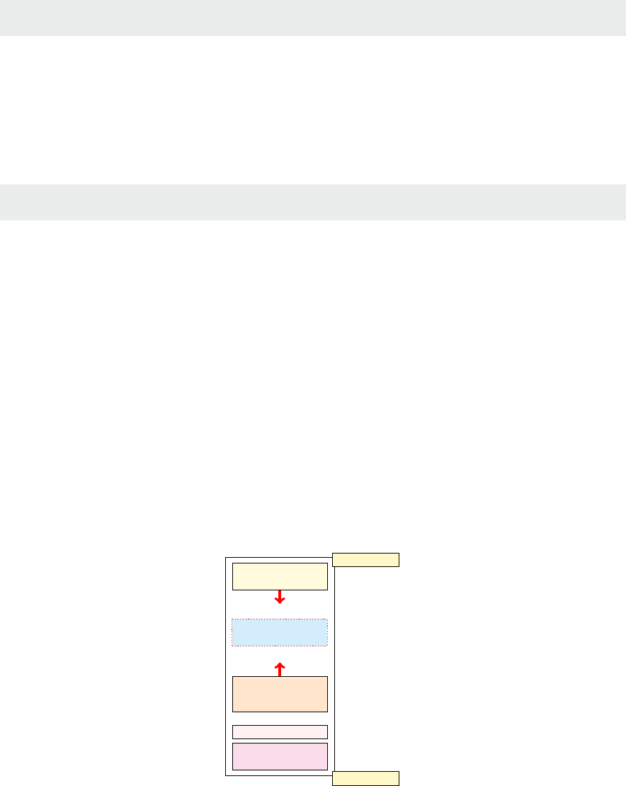
Operang Systems Foundaons with Linux on the Raspberry Pi
148
Check whether the OOM-killer is frequently invoked on your system with something like:
sudo cat /var/log/messages | grep "oom-killer"
Bash
6.6 Process view of memory
A process has the abstracon of logical memory spaces, which are superimposed on the paged virtual
address space as conguous segments. The text segment contains the program code. This is generally
loaded to known addresses by the runme loader, reading data from the stac ELF le. Text generally
starts at a known address. For instance, invoke:
ld --verbose | grep start
Bash
to nd this address for your system.
Data is usually located immediately aer the text. This includes stacally allocated data which may
be inialized (the data secon) or uninialized (the bss secon). The runme heap comes aer this
data. The runme stack, which supports funcon evaluaon, parameter passing, and scoped variables,
starts near the top of memory and grows downwards.
From a process perspecve, there are three ways in which the OS might add new pages to the virtual
address space while the program is running:
1. brk or sbrk extends the program break, eecvely growing the heap.
2. mmap allocates a new block of memory, possibly backed by a le.
3. The stack can grow down, as more funcons are called in a dynamically nested scope; the stack
expands on-demand, managed as part of the page fault handler.
Figure 6.14: Evoluon of a process’s user virtual address space, dynamic changes in red, lower addresses at the boom.
i
i
“chapter” — 2019/8/13 — 18:08 — page 15 — #15
i
i
i
i
i
i
stack
mmap()
heap
text
data
brk()
nested
calls
0
2GB or 3GB
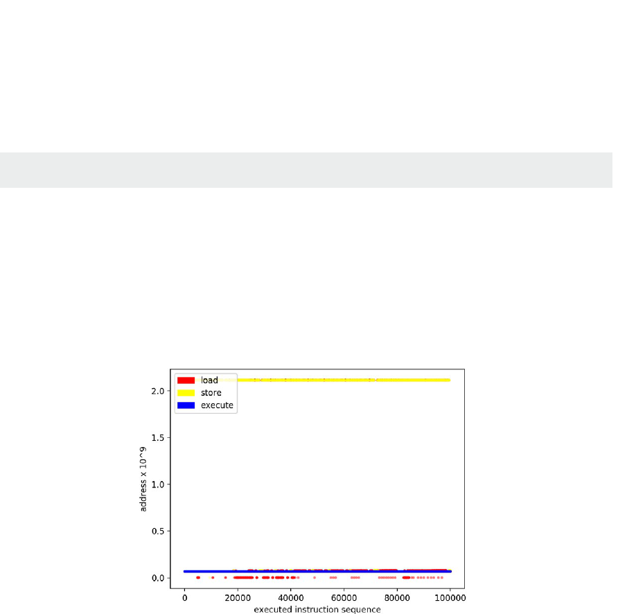
149
Figure 6.14 illustrates these three ways in which a process virtual address space may evolve. For a
more concrete example of process interacon with memory, we can use a tool like valgrind to trace
memory accesses at instrucon granularity. The visualizaons in Figure 6.15 show the sequence of
memory accesses recorded by valgrind for an execuon of the ls command. The precise command
used to generate the trace is:
valgrind --tool=lackey --trace-mem=yes ls
Bash
6.7 Advanced topics
There are several memory management techniques to improve system security and defend against
buer overow aacks. Address space layout randomizaon (ASLR) introduces random noise into the
locaons of executable code and runme memory areas like the stack and heap. This unpredictability
makes it more dicult for an aacker to vector to known code. The page metadata bit NX indicates
a page is not executable. Again, this migates code injecon aacks from user-input data.
Figure 6.15: Visualizaons of memory access paerns for an invocaon of the ls command, shown for rst 100,000 instrucons; the high red/yellow line is
the stack, the low blue line is the program executable text.
As single address space systems become larger, in terms of both the number of processor cores and
the amount of installed physical memory, there is increasing variance in memory access latency. One
reason for this is that some processor cores are located closer to parcular RAM chips; perhaps
a motherboard has several sockets, and integrated packages are plugged into each socket with RAM
and processor cores. This arrangement is referred to as non-uniform memory access or NUMA.
Figure 6.16 shows an example NUMA system, based on the Cavium ThunderX2 Arm processor
family. There are two NUMA regions (one per socket). Each region has tens of cores and a local bank
of RAM. Physical memory is mapped to pages, as outlined above. There is a single address space, so
every memory locaon is accessible from every core, but with dierent access latencies. Processor
i
i
“chapter” — 2019/8/13 — 18:08 — page 16 — #16
i
i
i
i
i
i
Chapter 6 | Memory management
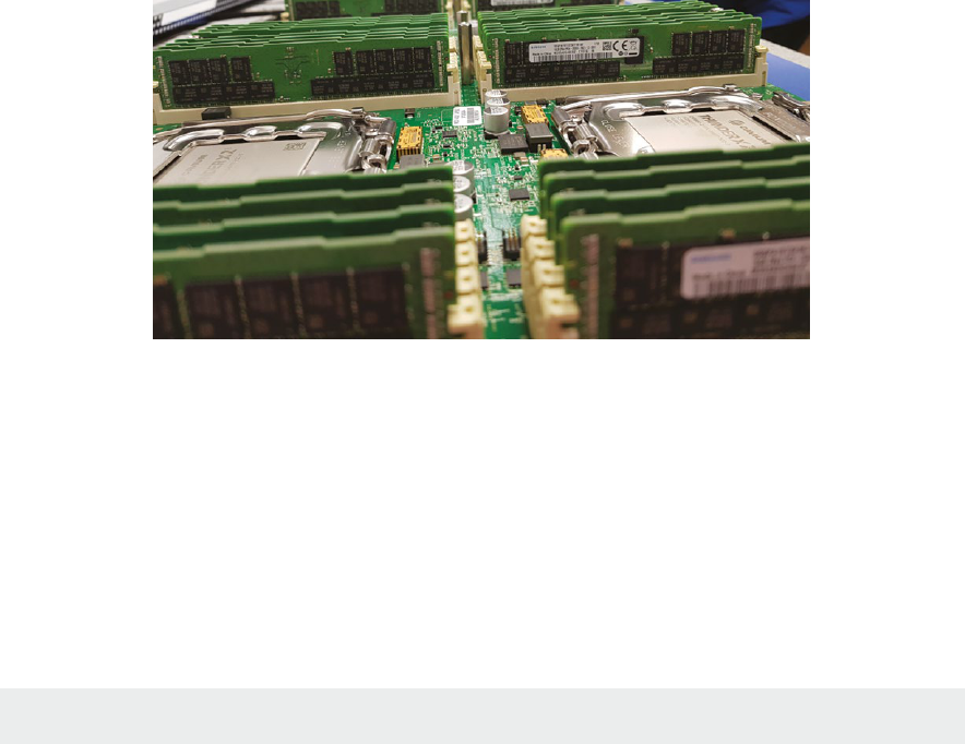
Operang Systems Foundaons with Linux on the Raspberry Pi
150
caches may hide some of the variance in memory access mes, but NUMA caching protocols are
complex. Writes to shared data can invalidate shared cache entries, forcing fresh data fetches from
main memory.
Figure 6.16 The Isambard HPC facility uses Cavium ThunderX2 NUMA processors which support mulple sockets with a shared address space; note the
disncve memory banks surrounding each processor package. Photo by Simon McIntosh-Smith.
Linux has several schemes to opmize memory access for NUMA architectures. Memory allocaon
may be interleaved, so it is placed in a round-robin fashion across all the nodes; this ensures memory
access mes are uniform on average, assuming an equal distribuon of probable accesses across the
address space. Another allocaon policy is node-local, which allocates memory close to the processor
execung the malloc; this assumes the memory is likely to be accessed by threads running on cores
in that same NUMA region.
You can determine whether your Linux system supports NUMA, by execung:
numactl --hardware
Bash
and see how many nodes are reported. Most Arm systems (in parcular, all Raspberry Pi boards) are
not NUMA. However, mulple socket motherboards will become increasingly common as core counts
increase, tracking Moore’s law in future years.
Another memory issue that aects large-scale servers, but may soon be apparent on smaller systems
is distributed memory. Protocols such as remote dynamic memory access (RDMA) enable pages to be
transferred rapidly from other machines to the local machine, copying memory from a remote buer
to a local buer with minimal OS intervenon. This is useful for migraon of processes or virtual
machines in cloud data centers. In more general terms, direct memory access (DMA) is a technique for
ecient copying of data between devices and memory buers. We will cover DMA in more detail in
Chapter 8 when we explore input/output. There is some addional complexity because many devices
work enrely in terms of physical memory addresses since they operate outside of the processor’s
virtual addressing domain.

151
Next-generaon systems may feature non-volale memory (NV-RAM). Whereas convenonal volale
RAM loses its data when the machine is powered down, NV-RAM persists data (like ash drives or
hard disks, but with faster access mes). NV-RAM is byte-addressable and oers signicant new
features for OSs, such as immediate restart of processes or enre systems, and full persistence for
in-memory databases.
6.8 Further reading
The Understanding the Linux Kernel textbook has helpful chapters on memory management, disk caches,
memory mapping, and swapping [1].
Gorman’s comprehensive documentaon on memory management in Linux [2] is a lile dated (based
on kernel version 2.6) but sll contains plenty of relevant and valuable material, including source code
commentary. It is the denive overview of the complex virtual memory management subsystem in
the Linux kernel.
Details of more recent kernel changes are available at the Linux Memory Management wiki,
hps://linux-mm.org.
To learn about Arm hardware support for memory management, consult Furber’s Arm System-on-Chip
textbook [3] for a generic overview, or the appropriate Arm architecture reference manual for specic
details.
6.9 Exercises and quesons
6.9.1 How much memory?
Calculate the size of your Raspberry Pi system’s virtual address space in megabytes by wring a short
C program.
Lisng 6.9.1: Compute the size of the virtual address space C
1 #include <stdio.h>
2 #include <sys/sysinfo.h>
3 #include <unistd.h>
4
5 int main() {
6 int pages = get_phys_pages();
7 int pagesize = getpagesize(); /* in bytes */
8 double ramGB = ((double)pages * (double)pagesize / 1024 / 1024 / 1024);
9 printf("RAM Size %.2f GB, Page Size %d B\n", ramGB, pagesize);
10 return 0;
11 }
How does the value reported compare with the system memory size stated by (a) /proc/meminfo
and (b) the ocial system documentaon? Can you account for any discrepancies?
Chapter 6 | Memory management
Operang Systems Foundaons with Linux on the Raspberry Pi
152
6.9.2 Hypothecal address space
Consider a 20-bit virtual address space, with pages of size 1KB.
1. Assuming byte-addressable memory, how many bits are required for a page/frame oset?
2. How many bits does this leave for specifying the page number?
3. Assume the page index bitstring is split into two equal porons, for rst-level and second-level page
table indexing. How many rst-level page tables should there be?
4. What is the maximum number of second-level page tables?
5. How many individual entries will there be in each page table?
6. What is the space overhead of this hierarchical page table, as opposed to a single-level page table,
when all pages are mapped to frames?
7. What is the space-saving of this hierarchical page table, as opposed to a single-level page table,
when only one page is mapped to a frame, i.e., there is a single entry in the page table mapping?
6.9.3 Custom memory protecon
The mprotect library funcon allows you to set page-level protecon (read, write, execute) for
allocated memory in user space. See man mprotect for more details. Sketch a scenario when
a developer may want to change page permissions:
1. From read/write to read-only, once a data structure has been inialized;
2. To make a page executable, once its data has been populated.
6.9.4 Inverted page tables
The simplest variant of an inverted page table contains one entry per frame. Each entry stores an
address space idener (ASID) to record which process is currently occupying this frame, along with
the virtual address corresponding to this physical address. Metadata permission bits may also be
stored with each entry. To look up a virtual address, it is only necessary to check whether the address
is present in any table entry—by looking up all table entries at once. This content-addressable approach
is how TLBs work since hardware support makes it possible to check all entries simultaneously.
1. What is the main problem with supporng inverted page tables enrely in soware, using an
in-memory data structure for the table?
2. Can you think of a more ecient soluon for inverted page table storage in soware?

153
6.9.5 How much memory?
Assume an OS is running p processes, and the plaorm has an n-level hierarchical page table. Each
node (including leaf nodes) in the page table occupies a single page. The page size is large enough to
store at least n address entries in a page table node:
1. How many pages would all the page tables occupy if each process has a single page of data in its
virtual address space?
2. What is the smallest number of pages occupied by all the page tables if each process has n pages
of data in its virtual address space?
3. What is the largest number of pages occupied by all the page tables if each process has n pages
of data in its virtual address space?
6.9.6 Tiny virtual address space
Imagine a system with an 8-bit, byte-addressable physical address space:
1. How many bytes of memory will there be?
2. For this system, consider using a virtual addressing scheme with single-level paging. If each page
contains 16 bytes, how many pages will there be?
3. In the worst case, what happens to memory access latency in a virtual addressing environments
with a single-level page table, with respect to physical addressing?
4. What could be done to migate this worst-case memory access latency?
5. In pracce, why is it unlikely that 8-bit memory would feature a virtual addressing scheme?
6.9.7 Denions quiz
Match the following concepts with their denions:
1. Swap le 1. Contains translaon data and protecon metadata for one or more pages.
2. Page table entry 2. When the OS perturbs regions of memory to ensure unpredictable
addresses for key data elements.
3. Thrashing 3. When a system cannot make useful progress since almost every memory
access requires pages to be swapped from the backing store.
4. MMU 4. Backing storage for pages that are not resident in memory.
5. Address space
randomizaon
5. A specialized hardware unit that maintains the abstracon of virtual
address spaces from the point-of-view of the processor.
Chapter 6 | Memory management

Operang Systems Foundaons with Linux on the Raspberry Pi
154
References
[1] D. P. Bovet and M. Cesa, Understanding the Linux Kernel, 3rd ed. O’Reilly, 2005.
[2] M. Gorman, Understanding the Linux Virtual Memory Manager. Prence Hall, 2004, hps://www.kernel.org/doc/gorman/
[3] S. Furber, ARM System-on-Chip Architecture, 2nd ed. Pearson, 2000.

155
Chapter 6 | Memory management

Chapter 7
Concurrency
and parallelism
Operang Systems Foundaons with Linux on the Raspberry Pi
158
7.1 Overview
In this chapter, we discuss how the OS supports concurrency, how the OS can assist in exploing
hardware parallelism, and how the OS support for concurrency and parallelism can be used to write
parallel and concurrent programs. We look at OS support for concurrent and parallel programming
via POSIX threads and present an overview of praccal parallel programming techniques such as
OpenMP, MPI, and OpenCL.
The exercises in this chapter focus on POSIX thread programming to explore the concepts of
concurrency, shared resource access and parallelism, and programming using OpenCL to expose the
student to praccal parallel heterogeneous programming.
What you will learn
Aer you have studied the material in this chapter, you will be able to:
1. Relate denions to the programmer’s view of concurrency and parallelism.
2. Discuss programming primives and APIs to handle concurrency and the OS and hardware support
for them.
3. Use the POSIX programming API to exploit parallelism and OS and hardware support for them.
4. Compare and contrast data- and task-parallel programming models.
5. Illustrate by example the popular parallel programming APIs.
7.2 Concurrency and parallelism: denions
To understand the implicaons and properes, rst of all, we need clear denions of concurrency
and parallelism.
7.2.1 What is concurrency?
Concurrency means that more than one task is running concurrently (at the same me) on the system.
In other words, concurrency is a property of the workload rather than the system, provided that the
system has support for running more than one task at the same me. In pracce, one of the key
reasons to have an OS is to support concurrency through scheduling of tasks on a single shared CPU.
7.2.2 What is parallelism?
Parallelism, by contrast, can be viewed as a property of the system: when a system has more than one
CPU core, it can execute several tasks in parallel, even if there is no scheduler to me-slice the tasks.
If the kernel supports hardware parallelism, it will try to speed up the execuon of tasks by making use
of the available parallel resources.
7.2.3 Programming model view
Another way of dening the terms parallelism and concurrency is as programming models. In praccal
terms, concurrent programming is about user experience and parallel programming about performance.
159
In a concurrent program, several threads of operaon are running at the same me because the user
expects several acons to be happening at the same me. For example, a web browser must at least
have a thread for networking, one for rendering the pages and one for user interacons (mouse clicks,
keyboard input). If these threads were not concurrent, the browser would not be usable.
By contrast, in a parallel program, what happens is that the work that would be performed on a single
CPU is split up and handed to mulple CPUs who execute each part in parallel. We can further disnguish
between task parallelism and data parallelism. Task parallelism means that every CPU core will perform a
dierent part of the computaon; for example, the steps in an image processing pipeline. Data parallelism
means that every CPU core will perform the same computaon but on a dierent part of the data. If we
run a parallel program on a single-core system, the only eect will be that it runs slower.
Because eecvely parallel programs execute concurrent threads, many of the issues of concurrent
programs are also encountered in parallel programming.
7.3 Concurrency
In this secon, we have a closer look at concurrency: the issues arising from concurrency and the techniques
to address them; support for concurrency in the hardware and the OS, and the POSIX programming API.
7.3.1 What are the issues with concurrency?
There are two factors which can lead to issues when several tasks are running concurrently: shared
resources and exchange of informaon between tasks.
Shared resources
When concurrent tasks share a resource, then access to that resource needs to be controlled to avoid
undesirable behavior. A very clear illustraon of this problem is a shared secon of railroad track, as
shown in Figure 7.1. Clearly, uncontrolled access could lead to disaster. Therefore, points in a railway
system are protected by semaphore signals. The single-track secon is the shared resource as it is
required by any trains traveling on the four tracks leading to it. When the signal indicates “Clear,” the
train can use the shared secon, at which point the signal will change to “Stop.” Any train wanng to
use the shared secon will have to wait unl the train occupying it has le, and the signal is “Clear”
again. We will discuss the OS equivalent in Secon 7.3.3.
Figure 7.1: Shared railroad track secon with points and semaphores.
Semaphore
Train
Points
(a)
(b)
Chapter 7 | Concurrency and parallelism
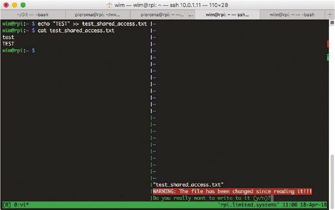
Operang Systems Foundaons with Linux on the Raspberry Pi
160
In a computer system, there many possible shared resources: le system, IO devices, memory. Let’s
rst consider the case of a shared le, e.g., a le in your home directory will be accessible by all
processes owned by you. Slightly simplifying, when a process opens a le, the le content is read into
the memory space of the process. When the process closes the le again, any changes will be wrien
back to disk. If two or more processes access the le concurrently for wring, there is a potenal for
conict: the changes made by the last process to write back to disk will overwrite all previous changes.
Therefore, most editors will warn if a le was modied by another process while open in the editor.
Figure 7.2: Concurrent access to a shared le using echo and vim.
For example, in Figure 7.2, I opened a le test_shared_access.txt in vim (right pane), and while
it was open, I modied it using echo (le pane). As you can see, when I then tried to save the le in
the editor, it warned me the le had been changed.
In the case of shared les, most operang systems leave the access control to the user. In the previous
example, before wring, vim checked the le on disk for changes. This is not possible for shared access
to IO devices because they are controlled by the operang system. In a way, this makes access control
easy because the OS can easily keep track of the processes using an IO resource. Shared access to
memory is more problemac. As we have seen, memory is not normally shared between processes;
each process has its own memory space. However, in a multhreaded process, the memory is shared
between all threads. In this case, again, the operang system leaves the access control to the user, i.e.,
the programmer of the applicaon. However, the operang system and the hardware provide support
for access control. The OS uses the hardware support to implement its internal mechanisms, and these
are used to implement the programmer API (e.g., POSIX pthreads).
Exchange of informaon
When concurrent tasks need to exchange informaon that is required to connue execuon, there
is a need to make sure that the sender either waits for the message (if it is sent late) or stores the
message unl needed (if it was sent early). Furthermore, if two or more tasks require informaon

161
from one another, care must be taken to avoid deadlock, i.e., the case where all tasks are waing for
the other tasks so no tasks can connue execuon. In the case of communicaon between threads
in a multhreaded process, the communicaon occurs via the shared memory. For communicaon
between processes, there are a number of possibilies, e.g., communicaon using shared les,
operang system pipes, network sockets, operang system message queues, or even shared memory.
The issues with the exchange of informaon in concurrent processes can be best explained using the
producer-consumer problem: each process is either a producer or a consumer of informaon. Ideally, any
item of informaon produced by a producer would be immediately consumed by a consumer. However,
in general, the rate of progress of producers and consumers is dierent (i.e., they are not operang
synchronously). Therefore, informaon needs to be buered, either by the consumer or by the producer.
In pracce buering capacity is always limited (the problem is therefore also known as the bounded buer
problem), so at some point, it is possible that the producer will have to suspend execuon unl there is
sucient buer capacity for the informaon to be produced. Note that in general there can be more than
one buer (e.g., it is common for each consumer to have a buer per producer).
Eecvely, the buer is a shared resource, so in terms of access control, informaon exchange, and
resource sharing are eecvely the same problem. This is also true for synchronizaon: the consumer
needs the informaon from the producer(s) in order to progress. So as long as that informaon is not
there, the producer has to wait. This is also the case with shared resources; for example, trains have
to wait unl the shared secon of track is free. In other words, control of access to shared resources
and synchronizaon of the exchange of informaon are just two dierent views on the same problem.
Consequently, there will be a single set of mechanisms that can be used to address this problem.
Note that if there are mulple producers and/or consumers, and a single shared resource, the problem is
usually known as the reader-writer problem, and has to address the concurrent access to the shared resource.
7.3.2 Concurrency terminology
When discussing synchronizaon and shared resources, it is useful to dene some addional terms
and concepts.
Crical secon
A crical secon for a shared resource is that poron of a program which accesses the resource
in such a way that mulple concurrent accesses would lead to undened or erroneous behavior.
Therefore, for a given shared resource, only one process can be execung its crical secon at
a me. The crical secon is said to be protected if the access to it is controlled in such a way that
the behavior is well-dened and correct.
Synchronizaon
In this context, by synchronizaon, we mean synchronizaon between concurrent threads of
execuon. When mulple processes need the exchange informaon, synchronizaon f the processes
results in a well-dened sequence of interacons.
Deadlock
Deadlock is the state in which each process in a group of communicang process is waing for
a message from the other process in order to proceed with an acon. Alternavely, in a group of
Chapter 7 | Concurrency and parallelism

Operang Systems Foundaons with Linux on the Raspberry Pi
162
processes with shared resources, there will be deadlock if each process is waing for another process
to release the resource that it needs to proceed with the acon.
A classic example of how the problem can occur is the so-called dining philosophers problem.
Slightly paraphrased, the problem is as follows:
Five philosophers sit around a round table with a bowl of noodles in front of each and a chopsck
between each of them.
Each philosopher needs two chopscks to eat the noodles.
Each philosopher alternately.
thinks for a while,
picks up two chopscks,
eats,
puts down the chopscks.
It is clear that there is potenal for deadlock here because there are not enough chopscks for all
philosophers to eat at the same me. If for example, they would all rst take the le chopsck, then
try to take the right one (or vice-versa), there would be deadlock. So how do they ensure there is no
deadlock?
Edsger Dijkstra (May 11, 1930 – Aug. 6, 2002) was a Dutch
computer scienst. He did his Ph.D. research from the University
of Amsterdam’s Mathemacal Center (1952–62). He taught and
researched at the Technical University of Eindhoven from 1963
to 1973 and at the University of Texas from 1984 onwards.
He was widely known for his 1959 algorithm that solves the
shortest-path problem. This algorithm is sll used to determine
the shortest path between two points, in parcular for roung
of communicaon net-works. In the course of his research on the
mutual exclusion in communicaons he suggested in 1962 the
concept of computer semaphores. His famous leer to CACM
in 1968, "Go To Statement Considered Harmful" was very inuenal
in the development of structured programming. He received the
Turing Award in 1972.
Image ©2002 Hamilton Richards
www.cs.utexas.edu/users/EWD/

163
7.3.3 Synchronizaon primives
In 1962, the famous Dutch computer scienst Edsger Dijkstra wrote a seminal – though interesngly,
technically unpublished – arcle tled “Over seinpalen” [1], i.e., “About Semaphores,” in which he
introduced the concept of semaphores as a mechanism to protect a shared resource. In Dijkstra’s
arcle, a semaphore S is a special type of shared memory, storing a non-negave integer. To access the
semaphore register, Dijkstra proposes two operaons, V(S), which stands for "verhoog,” i.e., increment,
and P(S), which stands for “prolaag,” i.e., try to decrement. The P(S) operaon will block unl the value
of S has been successfully decremented. Both operaons must be atomic.
If the semaphore can only take the values 0 or 1, Dijkstra specically menons the railway analogy,
where the V-operaon means “free the rail track” and the P-operaon “try to pass by the semaphore
onto the single track”, and that this is only possible if the semaphore is set to “Safe” and passing it
implies seng it to “Unsafe”.
Dijkstra calls a binary semaphore a mutex (mutual exclusion lock) [2]; a non-binary semaphore is
somemes called a counng semaphore. Although there is no general agreement on this denion,
the denions in the Arm Synchronizaon Primives Development Arcle [3] agree with this:
Mutex A variable, able to indicate the two states locked and unlocked. Aempng to lock a mutex already in
the locked state blocks execuon unl the agent holding the mutex unlocks it. Mutexes are somemes called
locks or binary semaphores.
Semaphore A counter that can be atomically incremented and decremented. Aempng to decrement
a semaphore that holds a value of less than 1 blocks execuon unl another agent increments the semaphore.
The key requirement of Dijkstra’s semaphores is the atomicity of the operaon. Modern processors
provide special atomic instrucons that allow implemenng semaphores eciently.
7.3.4 Arm hardware support for synchronizaon primives
Exclusive operaons and monitors
The ARMv6 architecture introduced the Load-Exclusive and Store-Exclusive synchronizaon
primives, LDREX and STREX, in combinaon with a hardware feature called exclusive monitor.
Quong from the Arm Synchronizaon Primives Development Arcle [3]:
LDREX The LDREX instrucon loads a word from memory, inializing the state of the exclusive monitor(s)
to track the synchronizaon operaon. For example, LDREX R1, [R0] performs a Load-Exclusive from the
address in R0, places the value into R1 and updates the exclusive monitor(s).
STREX The STREX instrucon performs a condional store of a word to memory. If the exclusive monitor(s)
permit the store, the operaon updates the memory locaon and returns the value 0 in the desnaon
register, indicang that the operaon succeeded. If the exclusive monitor(s) do not permit the store,
the operaon does not update the memory locaon and returns the value 1 in the desnaon register.
This makes it possible to implement condional execuon paths based on the success or failure of the
memory operaon. For example, STREX R2, R1, [R0] performs a Store-Exclusive operaon to the address
in R0, condionally storing the value from R1 and indicang success or failure in R2.
Chapter 7 | Concurrency and parallelism
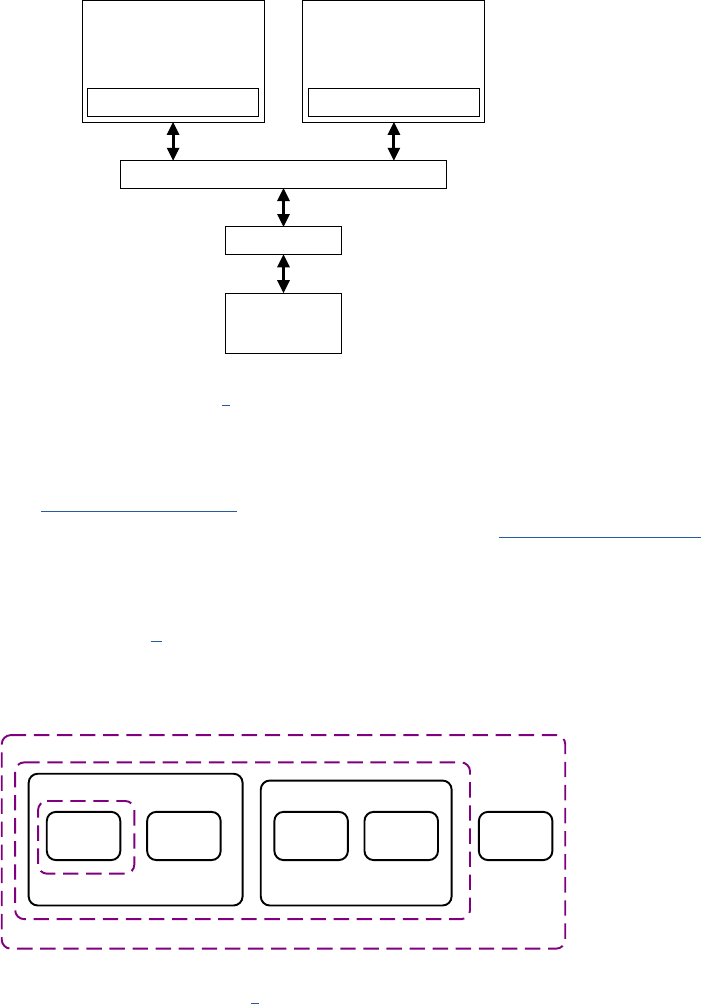
Operang Systems Foundaons with Linux on the Raspberry Pi
164
Exclusive monitors An exclusive monitor is a simple state machine, with the possible states open and exclusive.
To support synchronizaon between processors, a system must implement two sets of monitors, local and global
(Figure 7.3). A Load-Exclusive operaon updates the monitors to exclusive state. A Store-Exclusive operaon
accesses the monitor(s) to determine whether it can complete successfully. A Store-Exclusive can succeed only
if all accessed exclusive monitors are in the exclusive state.
Figure 7.3: Local and global monitors in a mul-core system (from [3]).
The LDREX and STREX instrucons are used by the Arm-specic Linux kernel code to implement the
kernel-specic synchronizaon primives which in their turn are used to implement POSIX synchronizaon
primives. For example, include/asm/spin lock.h implements spin lock funconality for the Arm
architecture, and this is used in the non-architecture-specic implementaon in include/linux/spin lock.h.
Shareability domains
In the context of cache-coherent symmetric mulprocessing (SMP), the Arm system architecture uses
the concept of shareability domains [4], which can be the Inner Shareable, Outer Shareable, System,
or Non-shareable , as illustrated in Figure 7.4. These domains are mainly used to restrict the range of
memory barriers, as discussed in Secon 7.3.5.
Figure 7.4: Shareability domains in an Arm manycore system, based on [5].
Cortex-A8
Local monitor
Cortex-R4
Local monitor
AXI interconnect
Global monitor
Memory
Core Core Core Core
Non-shareable
Inner shareable
Outer shareable
Processor Processor
GPU

165
The architectural denion of these domains is that they enable us to dene sets of observers for
which the shareability makes the data transparent for accesses. The Inner domain shares both code
and data, i.e., in pracce a mulcore system running an instance of an operang system will be in
the Inner domain; the Outer domain shares data but not code, and as shown in the gure could, for
example, contain a GPU, or a DSP or DMA engine. Marking a memory region as non-shareable means
that the local agent (core) does not share this region at all. This domain is not typically used in SMP
systems. Finally, if the domain is set to System, then an operaon on it aects all agents in the system.
For example, a UART interface would not normally be put in a shareable domain, so its domain would
be the full system.
7.3.5 Linux kernel synchronizaon primives
The Linux kernel implements a large number of synchronizaon primives; we discuss here only
a selecon.
Atomic primives
The Linux kernel implements a set of atomic operaons know as read-modify-write (RMW)
operaons. These are operaons where a value is read from a memory locaon, modied, and then
wrien back, with the guarantee that no other write will occur to that locaon between the read and
the write (hence the name atomic).
Most RMW operaons in Linux fall into one of two classes: those that operate on the special
atomic_t or atomic64_t data type, and those that operate on bitmaps, either stored in an
unsigned long or in an array of unsigned long.
The basic set of RMW operaons that are implemented individually for each architecture are known
as “atomic primives." As a kernel developer, you would use these to write architecture-independent
code such as a le system or a device driver.
As these primives work on atomic types or bitmaps, let’s rst have a look at these. The atomic types
are dened in types.h and they are actually simply integers wrapped in a struct:
Lisng 7.3.1: Linux kernel atomic types C
1 typedef struct {
2 int counter;
3 } atomic_t;
4
5 #ifdef CONFIG_64BIT
6 typedef struct {
7 long counter;
8 } atomic64_t;
9 #endif
The reason for this is that the atomic types should be dened as a signed integer but should also be
opaque so that a cast to a normal C integer type will fail.
Chapter 7 | Concurrency and parallelism

Operang Systems Foundaons with Linux on the Raspberry Pi
166
The simplest operaon on atomic types are inializaon, read and write, dened for the arm64
architecture in include/asm/atomic.h as:
Lisng 7.3.2: Linux kernel atomic type operaons (1) C
1 #dene ATOMIC_INIT(i) { (i) }
2
3 #dene atomic_read(v) READ_ONCE((v)->counter)
4 #dene atomic_set(v, i) WRITE_ONCE(((v)->counter), (i))
The READ_ONCE and WRITE_ONCE macros are dened in include/linux/compiler.h and are not
architecture-specic. Their purpose is to stop the compiler from merging or refetching reads or writes
or reordering occurrences of statements using these macros. We present them here purely to show
how non-trivial it is to stop a C compiler from opmizing.
Lisng 7.3.3: Linux kernel atomic type operaons (2) C
1 #include <asm/barrier.h>
2 #dene __READ_ONCE(x, check) \
3 ({ \
4 union { typeof(x) __val; char __c[1]; } __u; \
5 if (check) \
6 __read_once_size(&(x), __u.__c, sizeof(x)); \
7 else \
8 __read_once_size_nocheck(&(x), __u.__c, sizeof(x)); \
9 smp_read_barrier_depends(); /* Enforce dependency ordering from x */ \
10 __u.__val; \
11 })
12 #dene READ_ONCE(x) __READ_ONCE(x, 1)
13
14 #dene WRITE_ONCE(x, val) \
15 ({ \
16 union { typeof(x) __val; char __c[1]; } __u = \
17 { .__val = (__force typeof(x)) (val) }; \
18 __write_once_size(&(x), __u.__c, sizeof(x)); \
19 __u.__val; \
20 })
Bitmaps are, in a way simpler, as they are simply arrays of nave-size words. The Linux kernel provides
the macro DECLARE_BITMAP() to make it easier to create a bitmap:
Lisng 7.3.4: Linux kernel bitmap C
1 #dene DECLARE_BITMAP(name,bits) \
2 unsigned long name[BITS_TO_LONGS(bits)]
Here, BITS_TO_LONGS returns the number of words required to store the given number of bits.
The most common operaons on bitmaps are set_bit() and clear_bit() which for the arm64
architecture are dened in include/asm/bitops.h as:

167
Lisng 7.3.5: Linux kernel bitmap operaons (1) C
1 #ifndef CONFIG_SMP
2 / *
3 * The __* form of bitops are non-atomic and may be reordered.
4 */
5 #dene ATOMIC_BITOP(name,nr,p) \
6 (__builtin_constant_p(nr) ? ____atomic_##name(nr, p) : _##name(nr,p))
7 #else
8 #dene ATOMIC_BITOP(name,nr,p) _##name(nr,p)
9 #endif
10
11 / *
12 * Native endian atomic denitions.
13 */
14 #dene set_bit(nr,p) ATOMIC_BITOP(set_bit,nr,p)
15 #dene clear_bit(nr,p) ATOMIC_BITOP(clear_bit,nr,p)
16 }
The actual atomic operaons used in these macros are dened in include/asm/bitops.h as:
Lisng 7.3.6: Linux kernel bitmap operaons (2) C
1 / *
2 * These functions are the basis of our bit ops.
3 *
4 * First, the atomic bitops. These use native endian.
5 */
6 static inline void ____atomic_set_bit(unsigned int bit, volatile unsigned long *p)
7 {
8 unsigned longags;
9 unsigned long mask = BIT_MASK(bit);
10
11 p += BIT_WORD(bit);
12
13 raw_local_irq_save(ags);
14 *p |= mask;
15 raw_local_irq_restore(ags);
16 }
17
18 static inline void ____atomic_clear_bit(unsigned int bit, volatile unsigned long *p)
19 {
20 unsigned longags;
21 unsigned long mask = BIT_MASK(bit);
22
23 p += BIT_WORD(bit);
24
25 raw_local_irq_save(ags);
26 *p &= ~mask;
27 raw_local_irq_restore(ags);
28 }
The interesng point here is that the atomic behavior is achieved by masking the interrupt requests
and then restoring them, through the use of the architecture-independent funcons raw_local_
irq_save() and raw_local_irq_restore(). The architecture-specic implementaon of these
funcons for AArch64 is also provided in include/asm/bitops.h:
Chapter 7 | Concurrency and parallelism

Operang Systems Foundaons with Linux on the Raspberry Pi
168
Lisng 7.3.7: Atomic behavior through masking interrupt requests C
1 / *
2 * Aarch64 has ags for masking: Debug, Asynchronous (serror), Interrupts and
3 * FIQ exceptions, in the 'daif' register. We mask and unmask them in 'dai'
4 * order:
5 * Masking debug exceptions causes all other exceptions to be masked too/
6 * Masking SError masks irq, but not debug exceptions. Masking irqs has no
7 * side eects for other ags. Keeping to this order makes it easier for
8 * entry.S to know which exceptions should be unmasked.
9 */
10
11 / *
12 * CPU interrupt mask handling.
13 */
14 static inline unsigned long arch_local_irq_save(void)
15 {
16 unsigned longags;
17 asm volatile(
18 "mrs %0, daif // arch_local_irq_save\n"
19 "msr daifset, #2"
20 : "=r"(ags)
21 :
22 : "memory");
23 returnags;
24 }
25
26 / *
27 * restore saved IRQ state
28 */
29 static inline void arch_local_irq_restore(unsigned longags)
30 {
31 asm volatile(
32 "msr daif, %0 // arch_local_irq_restore"
33 :
34 : "r"(ags)
35 : "memory");
36 }
Masking interrupts is a simple and eecve mechanism to guarantee atomicity on a single-core
processor because the only way another thread could interfere with the operaon would be through
an interrupt. On a mulcore processor, it is in principle possible that a thread running on another core
would access the same memory locaon. Therefore, this mechanism is not useful outside the kernel.
If you use it in kernel code, it is assumed that you know what you’re doing, that is also why the rounes
have _local_ in their name, to indicate that they only operate on interrupts for the local CPU.
A nice overview of the API for operaons on atomic types can be found in the Linux kernel
documentaon in the les atomic_t.txt and atomic_bitops.txt. The operaons can be divided into
non-RMW and RMW. The former are read, set, read_acquire and set_release; the laer are arithmec,
bitwise, swap, and reference count operaons. Furthermore, each of these comes in an atomic_
and atomic64_ variant, as well as variants to indicate that there is a return value or not, and that the
fetched rather than the stored value is returned. Finally, they all come with relaxed, acquire, and
release variants, which need a bit more explanaon.

169
Memory operaon ordering
On a symmetric mulprocessing (SMP) system, accesses to memory from dierent CPUs are in principle
not ordered. We say that the memory operaon ordering is relaxed. Very oen, some degree of ordering
is required. The default for the Linux kernel is to impose a strict overall order via what is called a memory
barrier. Strictly speaking, a memory barrier imposes a perceived paral ordering over the memory operaons
on either side of the barrier. To quote from the Linux kernel documentaon (memory_barriers.txt),
Such enforcement is important because the CPUs and other devices in a system can use a variety of tricks
to improve performance, including reordering, deferral, and combinaon of memory operaons; speculave
loads; speculave branch predicon and various types of caching. Memory barriers are used to override or
suppress these tricks, allowing the code to sanely control the interacon of mulple CPUs and/or devices.
The kernel provides the memory barriers smp_mb {before,after}_atomic() and in pracce, the
strict operaon is composed of a relaxed operaon preceded and followed by a barrier, for example. Thus:
Lisng 7.3.8: Linux kernel atomic operaon through barriers C
1 atomic_fetch_add();
2 // is equivalent to :
3 smp_mb before_atomic();
4 atomic_fetch_add_relaxed();
5 smp_mb after_atomic();
Between relaxed and strictly ordered there are two other possible semancs, called acquire and release.
Acquire semancs applies to RMW operaons and load operaons that read from shared memory
(read-acquire), and it prevents memory reordering of the read-acquire with any read or write operaon
that follows it in program order.
Release semancs applies to RMW operaons and store operaons that write to shared memory
(write-release), and it prevents memory reordering of the write-release with any read or write operaon
that precedes it in program order.
Table 7.1 provides a summary of the possible cases.
Table 7.1: Memory operaon ordering semancs.
Type of operaon Ordering
Non-RMW operaons Unordered
RMW operaons
RMW operaons That have no return value Unordered
That have a return value Fully ordered
That have an explicit ordering
{operaon name}_relaxed Unordered
{operaon name}_acquire RMW read is an ACQUIRE
{operaon name}_release RMW write is a RELEASE
Chapter 7 | Concurrency and parallelism

Operang Systems Foundaons with Linux on the Raspberry Pi
170
Memory barriers
The memory barriers smp_mb {before,after}_atomic() are not the only types of barrier
provided by the Linux kernel. We can disnguish the following types [6]:
General barrier
A general barrier (barrier() from include/linux/compiler.h) has no eect at runme; it only serves
as an instrucon to the compiler to prevent reordering of memory accesses from one side of this
statement to the other. For the gcc compiler, this is implemented in the kernel code as
Lisng 7.3.9: Linux kernel general barrier C
1 #dene barrier() __asm__ __volatile__("": : :"memory")
Mandatory barriers
To enforce memory consistency on a full system level, you can use mandatory barriers. This is most
common when communicang with external memory-mapped peripherals. The kernel mandatory
barriers are guaranteed to expand to at least a general barrier, independent of the target architecture.
The Linux kernel has three basic mandatory CPU memory barriers:
GENERAL mb() A full system memory barrier. All memory operaons before the mb() in the instrucon
stream will be commied before any operaons aer the mb() are commied. This ordering will be visible to
all bus masters in the system. It will also ensure the order in which accesses from a single processor reaches
slave devices.
WRITE wmb() Like mb(), but only guarantees ordering between read accesses: all read operaons before
an rmb() will be commied before any read operaons aer the rmb().
READ rmb() Like mb(), but only guarantees ordering between write accesses: all write operaons before
a wmb() will be commied before any write operaons aer the wmb(). [6]
For the Arm AArch64 architecture, these barriers are implemented in arm64/include/asm/barrier.h as:
with the dsb() macro implemented in arm/include/asm/barrier.h as:
Lisng 7.3.10: Arm implementaon of kernel memory barriers (1) C
1 #dene mb() dsb(sy)
2 #dene rmb() dsb(ld)
3 #dene wmb() dsb(st)
with the dsb() macro implemented in arm/include/asm/barrier.h as:
Lisng 7.3.11: Arm implementaon of kernel memory barriers (2) C
1 #dene isb(option) __asm__ __volatile__ ("isb " #option : : : "memory")
2 #dene dsb(option) __asm__ __volatile__ ("dsb " #option : : : "memory")
3 #dene dmb(option) __asm__ __volatile__ ("dmb " #option : : : "memory")

171
Here, DMB, DSB, and ISB are respecvely Data Memory Barrier, Data Synchronizaon Barrier,
and Instrucon Synchronizaon Barrier instrucons [7]. In parcular, DSB acts as a special kind of
memory barrier. No instrucon occurring in the program order aer this instrucon executes unl this
instrucon has completed. The DSB instrucon completes when all explicit memory accesses before
this instrucon have completed (and all cache, branch predictor and TLB maintenance operaons
before this instrucon have completed).
The argument SY indicates a full system DSB operaon; LD is as DSB operaon that waits only for
loads to complete and ST is a DSB operaon that waits only for stores to complete.
SMP condional barriers
The SMP condional barriers are used to ensure a consistent view of memory between dierent cores
within a cache-coherent SMP system. When compiling a kernel without CONFIG_SMP, SMP barriers
are converted into plain general (i.e., compiler) barriers. Note that this means that SMP barriers cannot
replace a mandatory barrier, but a mandatory barrier can replace an SMP barrier.
The Linux kernel has three basic SMP condional CPU memory barriers:
GENERAL smp_mb() Similar to mb(), but only guarantees ordering between cores/processors within an SMP
system. All memory accesses before the smp_mb() will be visible to all cores within the SMP system before
any accesses aer the smp_mb().
WRITE smp_wmb() Like smp_mb(), but only guarantees ordering between read accesses.
READ smp_rmb() Like smp_mb(), but only guarantees ordering between write accesses. [6]
The SMP barriers are implemented in include/asm-generic/barrier.h as:
Lisng 7.3.12: Linux kernel SMP barriers C
1 #ifdef CONFIG_SMP
2 #ifndef smp_mb
3 #dene smp_mb() __smp_mb()
4 #endif
5 #ifndef smp_rmb
6 #dene smp_rmb() __smp_rmb()
7 #endif
8 #ifndef smp_wmb
9 #dene smp_wmb() __smp_wmb()
10 #endif
11 #endif
Chapter 7 | Concurrency and parallelism

Operang Systems Foundaons with Linux on the Raspberry Pi
172
For the Arm AArch64 architecture, the SMP barriers are implemented in arm64/include/asm/barrier.h as:
Lisng 7.3.13: Arm implementaon of kernel SMP barriers C
1 #dene __smp_mb() dmb(ish)
2 #dene __smp_rmb() dmb(ishld)
3 #dene __smp_wmb() dmb(ishst)
with the dmb() macro dened above.
DMB is the Data Memory Barrier instrucon. It ensures that all explicit memory accesses that appear
in program order before the DMB instrucon are observed before any explicit memory accesses
that appear in program order aer the DMB instrucon. It does not aect the ordering of any other
instrucons execung on the processor.
The argument ISH restricts a DMB operaon to the inner shareable domain; ISHLD is a DMB
operaon that waits only for loads to complete, and is restricted to inner shareable domain; ISHST
is a DMB operaon that waits only for stores to complete, and is restricted to the inner shareable
domain. Recall that the “inner shareable domain” is in pracce the memory space of the hardware
(SMP system) controlled by the Linux kernel.
Implicit barriers
Instead of explicit barriers, it is possible to use locking constructs available within the kernel that act
as implicit SMP barriers (similar to pthread synchronizaon operaons in user space, see Secon 7.3.6).
Because in pracce a large number of device drivers do not use the required barriers, the kernel I/O
accessor macros for the Arm architecture (readb(), iowrite32() etc.) act as explicit memory barriers
when the kernel is compiled with CONFIG_ARM_DMA_MEM_BUFFERABLE, for example in arm/
include/asm/io.h:
Lisng 7.3.14: Kernel I/O accessor macros for Arm as explicit memory barriers C
1 #ifdef CONFIG_ARM_DMA_MEM_BUFFERABLE
2 #include <asm/barrier.h>
3 #dene __iormb() rmb()
4 #dene __iowmb() wmb()
5 #else
6 #dene __iormb() do { } while (0)
7 #dene __iowmb() do { } while (0)
8 #endif
(the Linux kernel code uses do { } while (0) as an architecture-independent no-op).

173
Spin locks
Spin locks are the simplest form of locking. Essenally, the task trying to acquire the lock goes into
a loop doing nothing unl it gets the lock, in pseudocode:
Lisng 7.3.15: Spin lock pseudocode C
1 while (! has_lock ) {
2 // try to get the lock
3 }
Spin locks have the obvious drawback of occupying the CPU while waing. If the wait is long, another
task should get the CPU; in other words, the task trying to obtain the lock should be put to sleep.
However, for the cases where it is not desirable to put a task to sleep, or if the user knows the wait will
be short, the kernel provides spin locks, also known as busy-wait locks (kernel/locking/spin lock.c).
The spin lock funconality for SMP systems is implemented as a macro which creates a lock funcon
for a given operaon (e.g., read or write). Essenally, the implementaon is a forever loop with a
condional break. First, preempon is disabled, then the funcon tries to atomically acquire the lock,
and exits the loop if it succeeded; otherwise, it re-enables preempon and calls the architecture-
specic relax operaon, which eecvely is an ecient way of doing a no-op, and it performs another
iteraon of the loop and tries again.
Lisng 7.3.16: Linux kernel SMP lock-building macro C
1 #dene BUILD_LOCK_OPS(op, locktype) \
2 void __lockfunc __raw_##op##_lock(locktype##_t *lock) \
3 { \
4 for (;;) { \
5 preempt_disable(); \
6 if (likely(do_raw_##op##_trylock(lock))) \
7 break; \
8 preempt_enable(); \
9 \
10 arch_##op##_relax(&lock->raw_lock); \
11 } \
12 } \
For uniprocessor systems (include/linux/spin lock_api_up.h), the spin lock is much simpler:
Lisng 7.3.17: Linux kernel uniprocessor spin lock C
1 #dene ___LOCK(lock) \
2 do { __acquire(lock); (void)(lock); } while (0)
3
4 #dene __LOCK(lock) \
5 do { preempt_disable(); ___LOCK(lock); } while (0)
6
7 // ...
8 #dene _raw_spin_lock(lock) __LOCK(lock)
In other words, the code just disables preempon; there is no actual spin lock. The references to the
lock variable are there only to suppress compiler warnings.
Chapter 7 | Concurrency and parallelism

Operang Systems Foundaons with Linux on the Raspberry Pi
174
Futexes
As discussed in Secon 7.3.3, a mutex is a binary semaphore. A futex is a “fast user-space mutex,”
a Linux-specic implementaon of mutexes opmized for performance for the case when there is no
contenon for resources.
A futex (implemented in kernel/futex.c is idened by a user-space address which can be shared
between processes or threads. A basic futex has semaphore semancs: it is a 4-byte integer counter
that can be incremented and decremented only atomically; processes can wait for the value to become
posive. Processes can share this integer using mmap(2), via shared memory segments, or – if they are
threads – because they share memory space.
As the name suggests, futex operaon occurs enrely in user space for the non-contended case.
The kernel is only involved to handle the contended case. If the lock is already owned and another
process tries to acquire it then the lock is marked with a value that says, "waiter pending," and the
sys_futex(FUTEX_WAIT) syscall is used to wait for the other process to release it. The kernel
creates a ’futex queue’ internally so that it can, later on, match up the waiter with the waker – without
them having to know about each other. When the owner thread releases the futex, it noces (via the
variable value) that there were waiter(s) pending, and does the sys_futex(FUTEX_WAKE) syscall
to wake them up. Once all waiters have taken and released the lock, the futex is again back to the
uncontended state. At that point there is no in-kernel state associated with it, i.e., the kernel has no
memory of the futex at that address. This method makes futexes very lightweight and scalable.
Originally futexes, as described above, were used to implement POSIX pthread mutexes. However,
the current design is slightly more complicated due to the need to handle crashes. The problem is
that when a process crashes, it can’t clean up the mutex, but the kernel can’t do it either because it
has no memory of the futex. The changes required to address this issue are described in the kernel
documentaon in robust-futexes.txt.
Kernel mutexes
The Linux kernel also has its own mutex implementaon (mutex.h), which is intended for kernel-
use only (whereas the futex is designed for use by user-space programs). As usual, the kernel
documentaon (mutex-design.txt) is the canonical reference. Here we summarize the key points of the
implementaon. The mutex consists of the following struct:
Lisng 7.3.18: Linux kernel mutex struct C
1 struct mutex {
2 atomic_long_t owner;
3 spin lock_t wait_lock;
4 struct optimistic_spin_queue osq; /* Spinner MCS lock */
5 struct list_head wait_list;
6 };
The kernel mutex uses a three-state atomic counter to represent the dierent possible transions that
can occur during the lifeme of a lock: 1: unlocked; 0: locked, no waiters; <0: locked, with potenal
waiters

175
In its most basic form, it also includes a wait-queue and a spin lock that serializes access to it.
CONFIG_SMP systems can also include a pointer to the lock task owner as well as a spinner MCS lock
(see the kernel documentaon).
When acquiring a mutex, there are three possible paths that can be taken, depending on the state of
the lock:
1. Fastpath: tries to atomically acquire the lock by decremenng the counter. If it was already taken
by another task, it goes to the next possible path. This logic is architecture-specic but typically
requires only a few instrucons.
2. Midpath: aka opmisc spinning, tries to spin for acquision while the lock owner is running, and
there are no other tasks ready to run that have higher priority (need_resched). The raonale is that
if the lock owner is running, it is likely to release the lock soon.
3. Slowpath: if the lock is sll unable to be acquired, the task is added to the wait queue and
sleeps unl woken up by the unlock path. Under normal circumstances, it blocks as TASK_-
UNINTERRUPTIBLE.
While formally kernel mutexes are sleepable locks, it is the midpath that makes this lock aracve,
because busy-waing for a few cycles has a lower overhead than pung a task on the wait queue.
Semaphores
Semaphores (include/linux/semaphore.h) are also locks with blocking wait (sleep), they are a
generalized version of mutexes. Where a mutex can only have values 0 or 1, a semaphore can hold
an integer count, i.e., a semaphore may be acquired count mes before sleeping. If the count is zero,
there may be tasks waing on the wait_list. The spin lock controls access to the other members
of the semaphore. Unlike the mutex above, the semaphore always sleeps.
Lisng 7.3.19: Linux kernel semaphore struct C
1 struct semaphore {
2 raw_spin lock_t lock;
3 unsigned int count;
4 struct list_head wait_list;
5 };
The supported operaons on the semaphore (see kernel/locking/semaphore.c) are down (aempt to
acquire the semaphore, i.e., the P operaon) and up (release the semaphore, the V operaon). Both of
these have a number of variants, but we focus here on the basic versions.
Chapter 7 | Concurrency and parallelism

Operang Systems Foundaons with Linux on the Raspberry Pi
176
As long as the count is posive, down() simply decrements the counter:
Lisng 7.3.20: Linux kernel semaphore down() operaon (1) C
1 void down(struct semaphore *sem) {
2 unsigned long ags;
3
4 raw_spin_lock_irqsave(&sem->lock,ags);
5 if (likely(sem->count > 0))
6 sem->count--;
7 else
8 __down(sem);
9 raw_spin_unlock_irqrestore(&sem->lock,ags);
10 }
If no more tasks are allowed to acquire the semaphore, calling down() will put the task to sleep unl
the semaphore is released. This funconality is implemented in down() which simply calls down_
common (sem,TASK_UNINTERRUPTIBLE,MAX_SCHEDULE_TIMEOUT). The variable state refers
to the state of the current running process, as discussed in Chapter 5. The funcon adds the current
process to the semaphore’s wait list and goes into a loop. The trick here is that specifying a meout
value of MAX_SCHEDULE_TIMEOUT on schedule_meout() will call schedule() without a bound on the
meout. So this will simply put the current task to sleep. The return value will be MAX_SCHEDULE_
TIMEOUT.
Lisng 7.3.21: Linux kernel semaphore down() operaon (2) C
1 / *
2 * Because this function is inlined, the 'state' parameter will be
3 * constant, and thus optimized away by the compiler. Likewise the
4 * 'timeout' parameter for the cases without timeouts.
5 */
6 static inline int __sched __down_common(struct semaphore *sem, long state,
7 long timeout)
8 {
9 struct semaphore_waiter waiter;
10
11 list_add_tail(&waiter.list, &sem->wait_list);
12 waiter.task = current;
13 waiter.up = false;
14
15 for (;;) {
16 if (signal_pending_state(state, current))
17 goto interrupted;
18 if (unlikely(timeout <= 0))
19 goto timed_out;
20 __set_current_state(state);
21 raw_spin_unlock_irq(&sem->lock);
22 timeout = schedule_timeout(timeout);
23 raw_spin_lock_irq(&sem->lock);
24 if (waiter.up)
25 return 0;
26 }
27
28 timed_out:
29 list_del(&waiter.list);

177
30 return -ETIME;
31
32 interrupted:
33 list_del(&waiter.list);
34 return -EINTR;
35 }
The up() funcon is much simpler. It checks if there are no waiters, if so increments count, if not wakes
up the waiter at the head of the queue (using_up()).
Lisng 7.3.22: Linux kernel sempahore up() operaon (1) C
1 void up(struct semaphore *sem) {
2 unsigned longags;
3
4 raw_spin_lock_irqsave(&sem->lock,ags);
5 if (likely(list_empty(&sem->wait_list)))
6 sem->count++;
7 else
8 __up(sem);
9 raw_spin_unlock_irqrestore(&sem->lock,ags);
10 }
Lisng 7.3.23: Linux kernel semaphore up() operaon (2) C
1 static noinline void __sched __up(struct semaphore *sem)
2 {
3 structsemaphore_waiter*waiter=list_rst_entry(&sem->wait_list,
4 struct semaphore_waiter, list);
5 list_del(&waiter->list);
6 waiter->up = true;
7 wake_up_process(waiter->task);
8 }
7.3.6 POSIX synchronizaon primives
Unless you are a kernel or device driver programmer, you would not use the Linux kernel
synchronizaon primives directly. Instead, for userspace code, you would use the synchronizaon
primives provided by the POSIX API. These are implemented using the kernel primives discussed
above. The most important POSIX synchronizaon primives are mutexes, semaphores, spin lock,
and condion variables. The majority of the API is dened in <pthread.h>, with most of the types
in <sys/types.h>. The actual implementaon for Linux is the GNU C library glibc source code for,
see glibc.
Chapter 7 | Concurrency and parallelism

Operang Systems Foundaons with Linux on the Raspberry Pi
178
Mutexes
POSIX mutexes are dened as an opaque type pthread_mutex_t (eecvely a small integer). The API is
small and simple:
Lisng 7.3.24: POSIX mutex API C
1 //To create mutex:
2 pthread_mutex_t lock = PTHREAD_MUTEX_INITIALIZER;
3 // or
4 int pthread_mutex_init(pthread_mutex_t *mutex, const pthread_mutexattr_t *attr)
5
6 // To destroy a mutex:
7 int pthread_mutex_destroy(pthread_mutex_t *mutex);
8
9 //To lock/unlock the mutex:
10 int pthread_mutex_lock(pthread_mutex_t *lock);
11 int pthread_mutex_unlock(pthread_mutex_t *lock);
Semaphores
POSIX semaphores (dened in <semaphore.h>) are counng semaphores as introduced above, i.e.,
the block on an aempt to decrement them when the counter is zero. The Linux man page sem_-
overview(7) provides a good overview. The semaphore is dened using the opaque type semt_t.
The P and V operaons are called sem_wait() and sem_post():
Lisng 7.3.25: POSIX semaphore API C
1 // Separate header le, not in <pthread.h>
2 #include <semaphore.h>
3 // V operation
4 int sem_post(sem_t *sem);
5 // P operation
6 int sem_wait(sem_t *sem);
7 // Variants
8 int sem_trywait(sem_t *sem);
9 int sem_timedwait(sem_t *sem, const struct timespec *abs_timeout);
The sem_wait() variant sem_trywait() returns an error if the decrement cannot be immediately
performed instead of blocking. The variant sem_medwait() allows to set a meout on the waing
me. If the meout expires while the semaphore is sll blocked, an error is returned.
POSIX semaphores come in two forms: named semaphores and unnamed semaphores.
Named semaphores
A named semaphore is idened by a name of the form “/somename,” i.e., a null-terminated string
consisng of an inial slash, followed by one or more characters, none of which are slashes. Two
processes can operate on the same named semaphore by passing the same name to sem_open(). The
API consists of three funcons. The sem_open() funcon creates a new named semaphore or opens an
exisng named semaphore. When a process has nished using the semaphore, it can use sem_close()
to close the semaphore. When all processes have nished using the semaphore, it can be removed
from the system using sem_unlink().

179
Lisng 7.3.26: POSIX named semaphore API C
1 sem_t *sem_open(const char *name, intoag);
2 int sem_close(sem_t *sem);
3 int sem_unlink(const char *name);
Unnamed semaphores (memory-based semaphores)
An unnamed semaphore is placed in a region of memory that is shared between mulple threads
or processes. The API consists of three funcons. An unnamed semaphore must be inialized using
sem_init(). When the semaphore is no longer required, the semaphore should be destroyed using
sem_destroy().
Lisng 7.3.27: POSIX unnamed semaphore API C
1 int sem_init(sem_t *sem, int pshared, unsigned int value);
2 int sem_destroy(sem_t *sem);
Spin locks
POSIX spin locks are dened as an opaque type pthread_spin lock_t (eecvely a small integer). The
API consists of calls to inialize, destroy, lock, and unlock a spin lock. The trylock call tries to obtain
the lock and returns an error when it fails, rather than blocking.
Lisng 7.3.28: POSIX spin lock API C
1 // To create a spin lock
2 int pthread_spin_init(pthread_spin lock_t *, int);
3 // To destroy a spin lock
4 int pthread_spin_destroy(pthread_spin lock_t *);
5 // Get the lock
6 int pthread_spin_lock(pthread_spin lock_t *);
7 int pthread_spin_trylock(pthread_spin lock_t *);
8 // Release the lock
9 int pthread_spin_unlock(pthread_spin lock_t *);
Condion variables
Finally, the POSIX pthread API provides a more advanced locking construct called a condion variable.
Condion variables allow threads to synchronize based upon the actual value of data. Without
condion variables, the program would need to use polling to check if the condion is met, similar to
a spin lock. A condion variable allows the thread to wait unl a condion is sased, without polling.
A condion variable is always used in conjuncon with a mutex lock.
Below is a typical example of the use of condion variables. The code implements the basic operaons
for a thread-safe queue using an ordinary queue (Queue_t with methods enqueue(), dequeue() and
empty() and an aribute status), a mutex lock and a condion variable. The wait_- for_data() funcon
blocks on the queue as long as it is empty. The lock protects the queue q, and the pthread_cond_wait()
call blocks unl pthread_cond_signal() is called, in enqueue_data().
Chapter 7 | Concurrency and parallelism

Operang Systems Foundaons with Linux on the Raspberry Pi
180
Note that the call to pthread_cond_wait() automacally and atomically unlocks the associated mutex;
the mutex is automacally and atomically unlocked when receiving a signal.
The dequeue_data() method similarly protects the access to the queue with a mutex and uses the
condion variable to block unl the queue is non-empty. The funcons init(), and clean_up() are used
to create and destroy the mutex and condion variable.
Lisng 7.3.29: POSIX condion variable API C
1 pthread_mutex_t q_lock;
2 pthread_cond_t q_cond;
3
4 void init(pthread_mutex_t* q_lock_ptr,q_cond_ptr) {
5 pthread_mutex_init(q_lock_ptr,NULL);
6 pthread_cond_init(q_cond_ptr,NULL);
7 }
8
9 void wait_for_data(Queue_t* q) {
10 pthread_mutex_lock(&q_lock);
11 while(q->empty()) {
12 pthread_cond_wait(&q_cond, &q_lock);
13 }
14 q->status=1;
15 pthread_mutex_unlock(&q_lock);
16 }
17
18 void enqueue_data(Data_t* data, Queue_t* q) {
19 pthread_mutex_lock(&q_lock);
20 bool was_empty = (q->status==0);
21 q->enqueue(data);
22 q->status=1;
23 pthread_mutex_unlock(&q_lock);
24 if (was_empty)
25 pthread_cond_signal(&q_cond);
26 }
27
28 Data_t* dequeue_data(Queue_t* q) {
29 pthread_mutex_lock(&RXlock);
30 while(q->empty()) {
31 pthread_cond_wait(&RXcond, &RXlock);
32 }
33 Data_t* t_elt=q->front();
34 q->pop_front();
35 if (q->empty()) q->status=0;
36 pthread_mutex_unlock(&RXlock);
37 return t_elt;
38 }
39
40
41 void clean_up(pthread_mutex_t* q_lock_ptr,q_cond_ptr) {
42 pthread_mutex_destroy(q_lock_ptr);
43 pthread_cond_destroy(q_cond_ptr);
44 }
There is an addional API call pthread_cond_broadcast(). The dierence with pthread_cond_- signal() is
that the broadcast call unlocks all threads blocked on the condion variable, whereas the signal only
unlocks one thread.

181
POSIX condion variables are implemented in glibc for linux using futexes. The implementaon is
quite complex. The source code (nptl/pthread_cond_wait.c) contains an in-depth discussion of the
issues and design decisions. However, essenally, the implementaon can be wrien in Python
pseudocode as follows:
Lisng 7.3.30: POSIX condion variable pseudocode Python
1 def Condition(lock):
2 lock = Lock()
3 waitQueue = ThreadQueue()
4
5 def wait():
6 DisableInterrupts()
7 lock.release()
8 waitQueue.sleep()
9 lock.acquire()
10 RestoreInterrupts()
11
12 def signal():
13 DisableInterrupts()
14 waitQueue.wake()
15 RestoreInterrupts()
16
17 def broadcast():
18 DisableInterrupts()
19 waitQueue.wake-all()
20 RestoreInterrupts()
7.4 Parallelism
In this secon, we look at the hardware parallelism oered by modern architectures, the implicaons
for the OS and the programming support. For clarity, we will refer to one of several parallel hardware
execuon units as a “compute unit.” For example, in the Arm system shown in Figure 7.5, there would
be four quad-core A72 clusters paired with four quad-core A53 clusters, so a total of 32 compute units.
7.4.1 What are the challenges with parallelism?
The main challenge in exploing parallelism is in a way similar to scheduling: we want to use all
parallel hardware threads in the most ecient way. From the OS perspecve, this means control
over the threads to run on each compute unit. But whereas scheduling of threads/processes means
mulplexing in me, parallelism eecvely means the placement of tasks in space. The Linux kernel
has for a long me supported symmetric mulprocessing (SMP), which means an architecture where
mulple idencal compute units are connected to a single shared memory, typically via a hierarchy
of fully-shared, parally-shared and/or per-compute-unit caches. The kernel simply manages
a scheduling queue per core.
With the advent of systems like Arm’s big.LITTLE (of which the system in Figure 7.5 is an example,
with “big” A72 cores and “lile” A53 cores), this model is no longer adequate, because tasks will spend
a much longer me running if they are scheduled on a “lile” core than on a “big” core. Therefore
eorts have been started towards “global task scheduling” or “Heterogeneous mulprocessing” (HMP),
which require modicaons of the scheduler in the Linux kernel.
Chapter 7 | Concurrency and parallelism
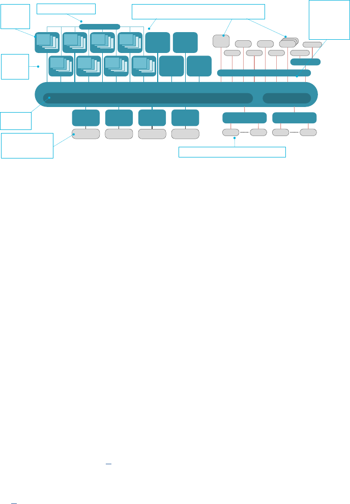
Operang Systems Foundaons with Linux on the Raspberry Pi
182
Figure 7.5: Extensible Architecture for Heterogeneous Mul-core Soluons (from ARM Tech Forum talk by Brian Je, September 2015).
Apart from these issues, there is also the issue of the control the user has over the placement of
tasks: ideally, the programmer should be able to decide on which compute unit a task should run.
This feature is known as “thread pinning” and supported by a POSIX API, and we will see how it is
implemented. Finally, parallel tasks on a shared memory system eecvely communicate via the
memory, which means that mulple concurrent accesses to the main memory are possible. This
poses challenges for cache coherency and TLB management, which are topics of Chapter 6, “Memory
management.” But even ignoring caches, communicaon eecvely means that the issues discussed
under the previous Secon on concurrency have to be addressed in parallel programs as well. The
main challenge is to ensure that there is no unnecessary sequenalizaon of tasks, while at the same
me guaranteeing that the resulng behavior is correct.
7.4.2 Arm hardware support for parallelism
When a processor comprises mulple processing cores, the hardware must be designed to support
parallel processing on all cores. Apart from supporng cache-coherent shared memory and the
features to support concurrency as discussed above, there are a few other ways in which Arm
mulcore processors support parallel programming. The rst is through SIMD (Single Instrucon
Mulple Data) instrucons, also known as vector processing. This type of parallelism does not require
intervenon from the OS as it is instrucon-based per-core parallelism, i.e., it is handled by the
compiler. The Arm Cortex-A53 MPCore Processor used in the Raspberry Pi 3 supports “Advanced
SIMD” extensions, as discussed in [8].
Next, the handling of interrupts must also be mul-core-aware. The Arm Generic Interrupt Controller
Architecture [9] provides support for soware control the delivery of hardware interrupts to a parcular
processing element (“Targeted distribuon model”) as well as to a one PE out of a given set (“1 of N
model”); and to control the delivery of soware interrupts to mulple PEs (“Targeted list model”).
Then we have support for processor anity through the Mulprocessor Anity Register, MPIDR. This
feature allows the OS to idenfy the PE on which a thread is to be scheduled.
DSP
DSP
ACE
Network Interconnect
NIC-400
Flash
NIC-400
USB
Memory
Controller
DMC-520
x72
DDR4-3200
AHB
Snoop Filter
1-32MB L3 cache
PCIe
10-40
GbE
DPI Crypto
CoreLink™ CCN-512 Cache Coherent Network
DSP
SATA
Memory
Controller
DMC-520
x72
DDR4-3200
Cortex-A72
Memory
Controller
DMC-520
x72
DDR4-3200
Memory
Controller
DMC-520
x72
DDR4-3200
PCIe
DPI
I/O Virtualisation CoreLink MMU-500
SRAM
Network Interconnect
NIC-400
GPIO
PCIe
GIC-500
Cortex CPU
or CHI
master
Cortex-A53
Cortex-A72
Cortex-A53
Cortex-A72
Cortex-A53
Cortex-A72
Cortex-A53
Cortex CPU
or CHI
master
Cortex CPU
or CHI
master
Cortex CPU
or CHI
master
®
Extensible Architecture for Heterogeneous Multi-core Solutions
Up to 4
cores per
cluster
Up to 12
coherent
clusters
Integrated
L3 cache
Up to 24 I/O
coherent
interfaces for
accelerators
and I/O
Peripheral address space
Heterogeneous processors – CPU, GPU, DSP and
accelerators
Virtualized Interrupts
Up to Quad
channel
DDR3/4 x72
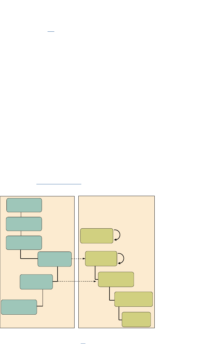
183
Finally, there are two hint instrucons [10] to improve mulprocessing, YIELD, and SEV. Soware
with a multhreading capability can use a YIELD instrucon to indicate to the PE that it is performing
a task, for example, a spin-lock, that could be swapped out to improve overall system performance.
The PE can use this hint to suspend and resume mulple soware threads if it supports the capability.
The Send Event (SEV) hint instrucon causes an event to be signaled to all PEs in the mulprocessor
system (as opposed to SEVL, which only signals to the local PE). The receipt of a singled SEV or SEVL
event by a PE sets the Event Register on that PE. The Event Register can be used by the Wait For
Event (WFE) instrucon. If the Event Register is set, the instrucon clears the register and completes
immediately; if it is clear, the PE can suspend execuon and enter a low-power state. It remains in that
state unl and SEV instrucon is executed by any of the PEs in the system.
7.4.3 Linux kernel support for parallelism
As menoned above, the Linux kernel supports parallelism through symmetric mulprocessing (SMP)
(ever since kernel version 2.0). What this means is that every compute unit runs a separate scheduler,
and there are mechanisms to move tasks between scheduling queues on dierent compute units.
SMP boot process
The boot process is, therefore extended from the boot sequence discussed in Chapter 2, as illustrated
in Figure 7.6. Essenally, the kernel boots on a primary CPU and when all common inializaon
is nished, the primary CPU sends interrupt requests to the other cores which result in running
secondary_start_kernel() (dened in arm/kernel/smp.c).
Figure 7.6: Boong owchart for the ARM Linux Kernel on SMP systems (from [11]).
Load balancing
The main mechanism to support parallelism in the Linux kernel is automac load balancing, which aims
to improve the performance of SMP systems by ooading tasks from busy CPUs to less busy or idle
Image Decompression
Primary CPU0 Secondary CPU 1, 2, 3,...
IDLE thread
IRQ
smp_init
Boot all secondary
CPUs by sending a
sync signal
Kernel_init (Process 1):
Initialize the SMP
environment and boot
all the secondary CPUs
start_kernel
(Process 0):
Initialization of all the
kernel components
Initialize the main
memory, cache, and
MMU specific to CPU0
cpu_up(cpu)
Wakeup and wait for
sync signal from CPU0
Execute WFI
(Wait For Interrupt)
Finalize initialization
and execute init
process to display
the console window
secondary_startup:
Initialize the memory,
cache, and MMU
specific to CPUx
secondary_start_kernel:
Initialize resources and
kernel structures specific
to CPUx
Wait for cpu_up(x)
from CPU0, where
x=current CPU
Wait for a signal
from CPU0
Chapter 7 | Concurrency and parallelism

Operang Systems Foundaons with Linux on the Raspberry Pi
184
ones. The Linux scheduler regularly checks how the task load is spread throughout the system and
performs load balancing if necessary [12].
To support load balancing, the scheduler supports the concepts of scheduling domains and groups
(dened in include/linux/sched/topology.h). Scheduling domains allow the grouping one or more
processors hierarchically for purposes load balancing. Each domain must contain one or more groups,
such that the domain consists of the union of the CPUs in all groups. Balancing within a domain occurs
between groups. The load of a group is dened as the sum of the load of each of its member CPUs,
and only when the load of a group becomes unbalanced are tasks moved between groups. The groups
are exposed to the user via two dierent mechanisms. The rst is autogroups, an implicit mechanism
in the sense that if it is enabled in the kernel (in /proc/sys/kernel/sched_autogroup_
enabled), all members of an autogroup are placed in the same kernel scheduler group. The second
mechanism is called control groups or cgroups (see cgroups(7)). These are not the same as the
scheduling task groups, but a way of grouping processes and control the resource ulizaon (including
CPU scheduling) at the level of the cgroup rather than at individual process level.
Processor anity control
The funconality used to move tasks between CPUs is exposed to the user using a kernel API dened
in include/linux/sched.h. This API consists of two calls (see sched_setanity(2)), sched_- setanity()
and sched_getanity().
Lisng 7.4.1: Linux processor anity control C
1 #dene _GNU_SOURCE
2 #include <sched.h>
3
4 int sched_setainity(pid_t pid, size_t cpusetsize,
5 const cpu_set_t *mask);
6
7 int sched_getainity(pid_t pid, size_t cpusetsize,
8 cpu_set_t *mask);
These calls control the thread’s CPU anity mask, which determines the set of CPUs on which it
can be run. On mulcore systems, this can be used to control the placement of threads. This allows
user-space applicaons to take control over the load balancing instead of the scheduler. Usually,
a programmer will not use the kernel API but the corresponding POSIX thread API (Secon 7.6.1),
which is implemented using the kernel API.
7.5 Data-parallel and task-parallel programming models
7.5.1 Data parallel programming
Data parallelism means that every compute unit will perform the same computaon but on a dierent
part of the data. This is a very common parallel programming model, supported for example by CPU
cores with SIMD vector instrucons, manycore systems, and GPGPUs.
Full data parallelism: map
Purely in terms of performance, in an ideal data-parallel program, the threads working on dierent
secons of the data would not interact at all. This type of problems is known as “embarrassingly

185
parallel.” In computaonal terms (especially in the context of funconal programming) this paern
is known as a map, a term which has become well-known through the popularity of map-reduce
frameworks. In principle, a map operaon can be executed on all elements of a data set in parallel,
so given unlimited parallelism, the complexity is O(1). In pracce, parallelism is never unlimited, and in
terms of implementaon of the map in programming languages, you cannot assume any parallelism,
for example, Python’s map funcon does not operate in parallel. However, we use the term here to
refer to the computaonal paern that allows full data parallelism.
Reducon
On the opposite side of the performance spectrum, we have purely sequenal computaons, i.e.,
where it is not possible at all to perform even part of the computaon in parallel. In computaonal
terms, this is the case for non-associave reducon operaons. Reducon (the second part in map-
reduce) means a computaon which combines all elements of a data set to produce its nal result.
In funconal programming, reducons are also known as folds. In Python, the corresponding funcon
is reduce. Unless a reducon operaon is associave, it cannot be parallelized and will have linear
me complexity O(N) for a data set of N elements.
Associavity
In formal terms, a funcon of two arguments is associave if and only if
f(f(x,y),z)=f(x,(f(y,z))
For example, addion and mulplicaon are associave:
x+y+z=(x+y)+z=x+(y+z)
but division and modulo are not:
(x/y)/z≠x/(y/z)
Binary tree-based parallel reducon
In pracce, many of the common operaons on sets are associave: sum, product, min, max,
concatenaon, comparison, ...
If the reducon operaon is associave, the computaon can sll be parallelized, not using a map
paern but through a binary tree-based parallelizaon (tree-based fold). For example, to sum 8
numbers, we can perform 4 pairwise sums in parallel, then sum the 4 results in two parallel operaons,
and then compute the nal sum.
1+2+3+4+5+6+7+8
= 3+7+11+15
= 10+26
= 36
Another example is merge sort, where the list to be sorted is split into as many chunks as there
are threads, then each chunk is sorted in parallel, and the chunks are merged pairwise. Whereas
Chapter 7 | Concurrency and parallelism
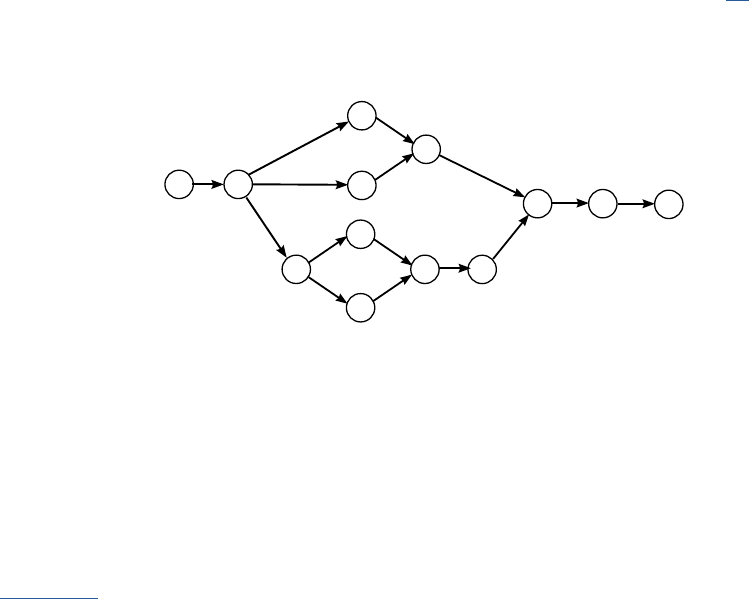
Operang Systems Foundaons with Linux on the Raspberry Pi
186
sequenal merge sort is O(N log N), if there are at least half as many threads as elements to sort, then
the sorng can be done in O(log N).
In general, for a data set of size N, with unlimited parallelism, an associave operaon can be reduced
in O(log N) steps.
7.5.2 Task parallel programming
Instead of parallelizing the computaon by performing the same operaon on dierent parts of the
data, we can also perform dierent computaons in parallel. For example, we can split a Sobel lter
for edge detecon in a vercal and horizontal part and perform these in parallel on the image data.
In pracce, this approach is parcularly eecve if the input data is a stream, e.g., frames from a video,
as in that case, we can create a pipeline which performs dierent operaons in parallel on dierent
frames. Figure 7.7 shows the complete task graph for a Sobel edge detecon pipeline [13]. In this
example, if a node has a fan-out of more than one, copies of the frame are sent to each downstream
node. In general, of course, a node could send dierent data to each of its downstream nodes.
Figure 7.7: Task graph for a Sobel edge detecon pipeline.
7.6 Praccal parallel programming frameworks
7.6.1 POSIX Threads (pthreads)
We have already covered the POSIX synchronizaon primives in Secon 7.3.6, but we did not
discuss the API for creang and managing threads. The POSIX thread (pthreads) API provides data
types and API calls to manage threads and control their aributes. A good overview can be found
in pthreads(7). The thread is represented by an opaque type pthread_t which represents the thread
ID (i.e., it is a small integer). Each thread has a number of aributes managed via the opaque type
pthread_ar_t, which is accessed via a separate set of API calls.
The most important thread management calls are pthread_create(), pthread_join() and pthread_- exit().
The pthread_create() call takes a pointer to the subroune to be called in the thread and a pointer to its
arguments. Inside the thread, pthread_exit() can be called to terminate the calling thread. The pthread_
join() call waits for the thread indicated by its rst argument to terminate, if that thread is in a joinable
state (see below). If that thread called pthread_exit() with a non-NULL argument, then this argument
will be available as the second argument in pthread_join().
video
frame
in
convert
to YCbCr
mirror
mirror
add
add
add
convert
from
YCbCr
Sobel-Hor
Sobel-Vert
Sobel-Hor
Sobel-Vert
video
frame
out

187
Lisng 7.6.1: POSIX pthread API: create and join C
1 #include <pthread.h>
2
3 int pthread_create(
4 pthread_t *thread, const pthread_attr_t *attr,
5 void *(*start_routine)(void*), void *arg);
6
7 int pthread_join(pthread_t thread, void **value_ptr);
8
9 // inside the thread
10 int pthread_exit(void *retval)
Another convenient call is pthread_self(), it simply returns the thread ID of the caller:
Lisng 7.6.2: POSIX pthread API: self C
1 pthread_t pthread_self(void);
In many cases, it is not necessary to specify the thread aributes, but we can use the aributes for
example to control the processor anity or the detached state of the thread, i.e., if a thread is joinable
or detached. Detached means that you know you will not use pthread_join() to wait for it, so on exit
the thread’s resources will be released immediately.
The aribute is created and destroyed using the following calls:
Lisng 7.6.3: POSIX pthread API: init and destroy C
1 int pthread_attr_init(pthread_attr_t *attr);
2 int pthread_attr_destroy(pthread_attr_t *attr);
For example, to set or get the anity, we can use the following calls:
Lisng 7.6.4: POSIX pthread API: anity C
1 #dene _GNU_SOURCE
2 int pthread_attr_setainity_np(pthread_attr_t *attr,
3 size_t cpusetsize, const cpu_set_t *cpuset);
4
5 int pthread_attr_getainity_np(pthread_attr_t
6 *attr, size_t cpusetsize, cpu_set_t *cpuset);
Similar, if we want to get or set the detach state we can use:
Lisng 7.6.5: POSIX pthread API: aributes C
1 int pthread_attr_setdetachstate(pthread_attr_t *attr, int detachstate);
2 int pthread_attr_getdetachstate(const pthread_attr_t *attr, int *detachstate);
Chapter 7 | Concurrency and parallelism

Operang Systems Foundaons with Linux on the Raspberry Pi
188
There are many more API calls both to manage the threads and the aributes, see the man page
pthreads(7) for more details.
Below is an example of typical use of pthreads to create a number of idencal worker threads to
perform work in parallel.
Lisng 7.6.6: POSIX pthread API example C
1 #include <pthread.h>
2
3 struct thread_info { /* Used as argument to thread_start() */
4 pthread_t thread_id; /* ID returned by pthread_create() */
5 // Any other eld you might need
6 // ...
7 };
8
9 // This is the worker which will run in each thread
10 void* thread_start(void *vtinfo) {
11 struct thread_info *tinfo = vtinfo;
12 // do work
13 // ...
14 pthread_exit(NULL); // no return value
15 }
16
17 int main(int argc, char *argv[]) {
18 int st;
19 struct thread_info *tinfo;
20 unsigned int num_threads = NTH; // macro
21
22 /* Allocate memory for pthread_create() arguments */
23 tinfo = calloc(num_threads, sizeof(struct thread_info));
24 if (tinfo == NULL)
25 handle_error("calloc");
26
27 /* Create threads (attr is NULL) */
28 for (unsigned int tnum = 0; tnum < num_threads; tnum++) {
29 // Here you would populate other elds in tinfo
30 st = pthread_create(&tinfo[tnum].thread_id, NULL,
31 &thread_start, &tinfo[tnum]);
32 if (st != 0)
33 handle_error_en(st, "pthread_create");
34 }
35
36 /* Now join with each thread */
37 for (unsigned int tnum = 0; tnum < num_threads; tnum++) {
38 st = pthread_join(tinfo[tnum].thread_id, NULL);
39 if (st != 0)
40 handle_error_en(st, "pthread_join");
41 }
42
43 // do something with the results if required
44 // ...
45
46 free(tinfo);
47 exit(EXIT_SUCCESS);
48 }
In this program, we create num_threads threads by calling pthread_create() in a for-loop (line 28).
Each thread is provided with a struct thread_info which contains the arguments for that thread.

189
Each thread takes a funcon pointer &thread_start to the subroune that will run in the thread.
The thread_info struct could, for example, contain a pointer to a large array, and each thread would
work on a poron of that array. As these threads are joinable (this is the default) we wait on them by
calling pthread_join() in a loop (line 37). Because the threads work on shared memory, the results of the
work done in parallel will be available in the main roune when all threads have been joined.
7.6.2 OpenMP
OpenMP is the de-facto standard for shared-memory parallel programming. It is based on a set
of compiler direcves or pragmas, combined with a programming API to specify parallel regions,
data scope, synchronizaon, etc.. OpenMP is a portable parallel programming approach, and the
specicaon supports C, C++, and Fortran. It has been historically used for data-parallel programming
through its compiler direcves. Since version 3.0, OpenMP also supports task parallelism [14]. It is
now widely used in both task and data parallel scenarios. Since OpenMP is a language enhancement,
every new construct requires compiler support. Therefore, its funconality is not as extensive as
library-based models. Moreover, although OpenMP provides the user with a high level of abstracon,
the onus is sll on the programmer to ensure proper synchronizaon.
A typical example of OpenMP usage is the parallelizaon of a for-loop, as shown in the following code
snippet:
Lisng 7.6.7: OpenMP example C
1 #include <omp.h>
2 // ...
3 #pragma omp parallel \
4 shared(collection,vocabulary) \
2 private(docsz_min,docsz_max,docsz_mean)
6 {
7 // ...
8 #pragma omp for
9 for (unsigned int docid = 1; docid<NDOCS; docid++) {
10 // ...
11 }
12 }
The #pragma omp for direcve will instruct the compiler to parallelize the loop (using POSIX
threads), treang it eecvely as a map. The shared() and private() clauses in the #pragma omp parallel
direcve let the programmer idenfy which variables are to be treated as shared by all threads or
private (per-thread). However, this clause does not regulate access to the variables, so we require
some kind of access control. OpenMP provides a number of direcves to control access to secons
of code, the most important of which correspond to concepts introduced earlier:
#pragma omp crical indicates a crical secon, i.e., it species a region of code that must be
executed by only one thread at a me.
#pragma omp atomic indicates that a specic memory locaon must be updated atomically, rather
than leng mulple threads aempt to write to it. Essenally, this direcve provides a single-
statement crical secon.
Chapter 7 | Concurrency and parallelism

Operang Systems Foundaons with Linux on the Raspberry Pi
190
#pragma omp barrier indicates a memory barrier; a thread will wait at that point unl all other threads
have reached that barrier. Then, all threads resume parallel execuon of the code following aer
the barrier.
For a full descripon of all direcve-based OpenMP synchronizaon constructs, see the OpenMP
specicaon [15]. In some cases, the direcve-based approach might not be suitable. Therefore
OpenMP also provides an API for synchronizaon, similar to the POSIX API. The following snippet
illustrates the use of locks to protect a crical secon.
Lisng 7.6.8: OpenMP lock example C
1 omp_lock_t writelock;
2 #pragma omp parallel \
3 shared(collection,vocabulary) \
4 private(docsz_min,docsz_max,docsz_mean)
5 {
6 omp_init_lock(&writelock);
7 #pragma omp for
8 for (unsigned int docid = 1; docid<NDOCS; docid++) {
9 // ...
10 omp_set_lock(&writelock);
11 // shared access
12 // ...
13 omp_unset_lock(&writelock);
14 }
15 omp_destroy_lock(&writelock);
16 }
7.6.3 Message passing interface (MPI)
The Message Passing Interface (commonly known under its acronym MPI) [16] is an API specicaon
designed for high-performance compung. Since MPI provides a distributed memory model for
parallel programming, its main targets have been clusters and mulprocessor machines. The message
passing model means that tasks do not share any memory. Instead, every task has its own private
memory, and any communicaon between tasks is via the exchange of messages.
In MPI, the two basic rounes for sending and receiving messages are MPI_Send and MPI_- Recv:
Lisng 7.6.9: MPI send and receive API C
1 int MPI_Send(const void *buf, int count, MPI_Datatype datatype, int dest, int tag,
2 MPI_Comm comm)
3 int MPI_Recv(void *buf, int count, MPI_Datatype datatype, int source, int tag,
4 MPI_Comm comm, MPI_Status *status)
The buer buf contains the data to send or receive, the count its size in mulples of the specied
datatype. Further arguments are the desnaon (for send) or source (for receive). These are usually
called ranks, i.e. “a sender with rank X sends to a receiver with rank Y.” The two remaining elds, tag,
and communicator, require a bit more detail.
The communicator is essenally an object describing a group of processes that can communicate
with one another. For simple problems, the default communicator MPI_COMM_WORLD can be used,
but custom communicators allow, for example, collecve communicaon between subsets of all
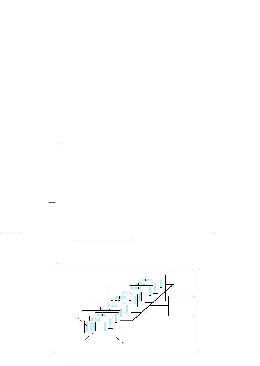
191
processes. An important point is that the rank of a process is specic to the communicator being used,
i.e., the same process will typically have dierent ranks in dierent communicators.
The tag is an arbitrary integer that is used for matching of point-to-point messages like send and
receive: if a sender sends a message to a given desnaon with rank dest with a communicator
comm and a tag tag, then the receiver must match all of these specicaons in order to receive the
message, i.e., it must specify comm as its communicator, tag for its tag (or the special wildcard MPI_
ANY_TAG), and the rank of the sender as the source (or the special wildcard MPI_ANY_- SOURCE).
The MPI specicaon has evolved considerably since its inial release in 1994. For example, MPI-
1 already provided point-to-point and collecve message communicaon. Messages could contain
either primive or derived data types in packed or unpacked data content. MPI-2 added dynamic
process creaon, one-sided communicaon, remote memory access, and parallel I/O.
Since there are lots of MPI implementaons with emphasizes on dierent aspects of high-performance
compung, Open MPI [17], an MPI-2 implementaon, evolved to combine these technologies and
resources with the main focus on the components concepts. The specicaon is very extensive, with
almost 400 API calls.
MPI is portable, and in general, an MPI program can run on both shared memory and distributed
memory systems. However, for performance reasons and due to the distributed nature of the model,
there might exist mulple copies of the global data in a shared memory machine, resulng in an
increased memory requirement. Message buers also introduce the overhead of MPI on shared-
memory plaorms [18]. Furthermore, because the API is both low level and very extensive, MPI
programming, especially for performance, tends to be complicated.
7.6.4 OpenCL
OpenCL is an open standard for parallel compung using heterogeneous architectures [19]. Arm provides
an implementaon as part of the Compute Library One of the main objecves of OpenCL is to increase
portability across dierent plaorms and devices, e.g., GPUs, mulcore processors, and other accelerators
such as FPGAs, as well as across operang systems. OpenCL provides an abstract plaorm model and an
abstract device model [20]. The plaorm (Figure 7.8) consists of a host and a number of compute devices.
Figure 7.8: OpenCL plaorm model (from [20]).
Compute Unit
...
...
...
...
...
...
...
...
...
...
...
...
Compute Device
Processing
Element
Host
Chapter 7 | Concurrency and parallelism
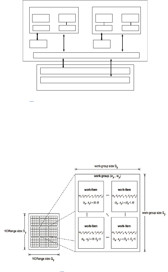
Operang Systems Foundaons with Linux on the Raspberry Pi
192
Each compute device (Figure 7.9) consists of a number of compute units which each comprise a number
of processing elements. All compute units can access the shared compute device memory (which consists
of a global and a constant memory), oponally via a shared cache; each compute unit has local memory
accessible by all processing elements, and private memory per processing element.
Figure 7.9: OpenCL device model (from [20]).
The programming framework of OpenCL consists of an API for controlling the operaon of
the devices and transfer of data and programs between the host memory and the device memory, and
a language for wring kernels (the programs running on the devices) based on C99, with the following
restricons: no funcon pointers; no recursion; no variable-length arrays; no irreducible control ow.
Furthermore, as it is assumed that memory space of the compute device is not under control of the
host OS and that it does not run its own OS, system calls are not supported either. These restricons
originate from the nature of typical OpenCL devices, in parcular, GPUs.
Figure 7.10: NDRanges, work-groups and work-items (from [20]).
Compute Device
Compute unit 1 Compute unit N
Private
memory 1
Private
memory M
PE 1 PE M
Private
memory 1
Private
memory M
PE 1 PE M
Local
memory 1
Local
memory N
Global/Constant Memory Data Cache
Global Memory
Constant Memory
Compute Device Memory
...
...
...

193
Although OpenCL supports task-parallel programming, its main model is data parallelism. To divide
a data space over the compute units and processing elements, OpenCL provides the concepts of the
n-dimensional range (NDRange), work-groups and work-items, as illustrated in Figure 7.10 for a 2-D
space. The NDRange species how many threads will be used to process the data set. Note that this
can be larger than the actual number of hardware threads, in which case OpenCL will schedule the
threads on the available hardware. The NDRange can be further split into a global range and a local
range. To illustrate this usage, consider a 1-D case for a device with 16 compute units which each have
128 threads, and we want to map exactly one hardware thread per element in the NDRange. In that
case, the global NDRange will be 16*128 and the local NDRange 128. Now assume that the data to
be processed is an array of 64M words, then we have to process 32,768 elements per hardware
thread. We can use the global NDRange index and global size to idenfy which poron of the array
a thread must process, as shown in the following code snippet:
Lisng 7.6.10: OpenCL example C
1 // aSize is the size of array, i.e. 64M
2 __kernel square(__global oat* a, __global oat a_squared, const int aSize) {
3
4 int gl_id = get_global_id(0); // 0 .. 16*128-1
5 int gSize = get_global_size(0); // 16*128
6 // alternatively
7 int n_groups = get_num_groups(0); // 16
8 int l_id = get_local_id(0); // 0 .. 127
9 int gr_id = get_group_id(0); // 0 .. 15
10
11 int wSize = aSize/gSize; // 32,768
12
13 int start = gl_id*wSize;
14 int stop = (gl_id+1)*wSize;
15 for (int idx = start; idx<stop; idx++) {
16 a_squared[idx]=a[idx]*a[idx];
17 }
18 }
Alternavely we could use the local NDRange index, group index and number of workgroups, the
relaonship is as follows:
work_group_size = global_size/number_of_work_groups
global_id = work_group_id*work_group_size+local_id
Chapter 7 | Concurrency and parallelism

Operang Systems Foundaons with Linux on the Raspberry Pi
194
The OpenCL host API is quite large and ne-grained; we refer the reader to the specicaon [20].
We have created a library called oclWrapper
1
to simplify OpenCL host code for the most common
scenarios. Using this wrapper, typically a program looks like this:
Lisng 7.6.11: OpenCL wrapper example C
1 // Create wrapper for default device and single kernel
2 OclWrapper ocl(srclename,kernelname,opts);
3
4 // Create read and write buers
5 cl::Buerrbuf=ocl.makeReadBuer(sz);
6 cl::Buerwbuf=ocl.makeWriteBuer(sz);
7
8 // Transfer input data to device
9 ocl.writeBuer(rbuf,sz,warray);
10
11 // Set up index space
12 ocl.enqueueNDRange(globalrange, localrange);
13
14 // Run kernel
15 ocl.runKernel(wbuf,rbuf ).wait();
16
17 // Read output data from device
18 ocl.readBuer(wbuf,sz,rarray);
First, we create an instance of the OclWrapper class, which is our abstracon for the OpenCL host
API. The constructor takes the kernel le name, kernel name and some opons, e.g., to specify which
device to use. Then we create buers, these are objects used by OpenCL to manage the transfer of
data between host and device. Then we transfer the input data for the device (via what in OpenCL is
called the read buer). Then we set up the NDRange index space, and run the kernel. Finally, we read
the output data (through what OpenCL calls the write buer).
7.6.5 Intel threading building blocks (TBB)
Intel threading building blocks (TBB) is an open-source, object-oriented C++ template library
for parallel programming originally developed by Intel [21, 22]. It is not specic to the Intel CPU
architecture and works well on the Arm architecture
2
, because it is implemented using the POSIX
pthread API. Intel TBB contains several templates for parallel algorithms, such as parallel_for and
parallel_reduce. It also contains useful parallel data structures, such as concurrent_vector
and concurrent_queue. Other important features of the Intel TBB are its scalable memory allocator
as well as its primives for synchronizaon and atomic operaons.
TBB abstracts the low-level threading details. However, the tasking comes along with an overhead.
Conversion of the legacy code to TBB requires restructuring certain parts of the program to t the
TBB templates. Moreover, there is a signicant overhead associated with the sequenal execuon
of a TBB program, i.e., with a single thread [23].
1
hps://github.com/wimvanderbauwhede/OpenCLIntegraon
2
There is currently no tbb package in Raspbian for the Raspberry Pi 3. However, it is easy to build tbb from source, using the following command: make tbb CXXFLAGS="-
DTBB_USE_GCC_BUILTINS=1 -D TBB_64BIT_- ATOMICS=0"

195
A task is the central unit of execuon in TBB, which is scheduled by the library’s runme engine. One
of the advantages of TBB over OpenMP is that it does not require specic compiler support. TBB is
based enrely on runme libraries.
7.6.6 MapReduce
MapReduce, originally developed by Google [24], has become a very popular model for processing
large data sets, especially on large clusters (cloud compung). The processing consists of paroning
the dataset to be processed and dening map and reduce funcons. The map funconality is
responsible for parallel processing of a large volume of data and generang intermediate key-value
pairs. The role of the reduce funconality is to merge all the intermediate values with the same
intermediate key.
Because of its simplicity, MapReduce has quickly gained in popularity. The paroning,
communicaon and message passing, and scheduling across dierent nodes are all handled by the
runme system so that the user only has to express the MapReduce semancs. However, its use is
limited to scenarios where the dataset can be operated on in embarrassingly parallel fashion. The
MapReduce specicaon does not assume a shared or distributed memory model. Although most of
the implementaons have been on large clusters, there has been work on opmizing it for mulcores
[25]. Popular implementaons of the MapReduce model are Spark and Hadoop.
7.7 Summary
In this chapter, we have introduced the concepts of concurrency and parallelism, explained the
dierence between them and looked at why both are essenal in modern computer systems. We have
studied at how the Arm hardware architecture and the Linux kernel handle and support concurrency
and parallelism. In parcular, we have discussed the synchronizaon primives in the kernel (atomic
operaons, locks, semaphores, barriers, etc.) and how they rely on hardware features; we have also
looked at the kernel support for parallelism, in parcular in terms of the scheduler and the control over
the placement of threads.
We have introduced the data-parallel and task-parallel programming models and briey discussed
a number of popular praccal parallel programming frameworks.
7.8 Exercises and quesons
1. Implement a soluon to the dining philosophers problem in C using the POSIX threads API.
2. Create a system of N threads that communicate via stac arrays of size N dened in each thread,
using condion variables and mutexes.
3. Write a data-parallel program that produces the sum of the squares of all values in an array, using
pthreads and using OpenMP.
Chapter 7 | Concurrency and parallelism
Operang Systems Foundaons with Linux on the Raspberry Pi
196
7.8.1 Concurrency: synchronizaon of tasks
1. What is a crical secon? When is it important for a task to enter a crical secon?
2. Could a task be pre-empted while execung its crical secon?
3. What is the dierence between a semaphore and a mutex?
4. What is a spin lock, and what are its properes, advantages and disadvantages?
5. Sketch the operaons required for two tasks using semaphores to perform mutual exclusion of
a crical secon, including semaphore inializaon.
6. Sketch the operaons required to synchronize two tasks, including semaphore inializaon.
7. Specify the possible order of the code executed by two tasks synchronized using semaphores,
running on a uniprocessor system.
8. What Pthreads concept is provided to enable meeng such synchronizaon requirements? Sketch
how a typical task uses this concept in pseudocode.
9. Sketch the pseudocode for the typical use of POSIX condion variables and mutexes to implement
a thread-safe queue.
10. Explain the concept of shareability domains in the Arm system architecture
7.8.2 Parallelism
1. Discuss the hardware support for parallelism in Arm mulcore processors.
2. What is processor anity, and how can controlling it benet your parallel program?
3. Given unlimited parallelism, what is the big-O complexity for a merge sort? And what is it given
limited parallelism?
4. Explain the OpenCL model of data-parallelism.
5. When would you call pthread_exit() instead of exit()?

197
References
[1] E. W. Dijkstra, “Over seinpalen,” 1962, circulated privately. [Online].
Available: hp://www.cs.utexas.edu/users/EWD/ewd00xx/EWD74.PDF
[2] ——, “A tutorial on the split binary semaphore,” Mar. 1979, circulated privately. [Online].
Available: hp://www.cs.utexas.edu/users/EWD/ewd07xx/EWD703.PDF
[3] Arm Synchronizaon Primives Development Arcle, Arm Ltd, 8 2009, issue A. [Online].
Available: hp://infocenter.arm.com/help/index.jsp?topic=/com.arm.doc.dht0008a/index.html
[4] L. Lindholm, “Memory access ordering part 2 - memory access ordering in the Arm Architecture,” 2013. [Online].
Available: hps://community.arm.com/processors/b/blog/posts/memory-access-ordering-part-3---memory-access-ordering-in-
the-arm-architecture
[5] Arm Cortex-A Series - Programmer’s Guide for ARMv8-A - Version: 1.0, Arm Ltd, 3 2015, issue A. [Online].
Available: hp://infocenter.arm.com/help/topic/com.arm.doc.den0024a/DEN0024A_v8_architecture_PG.pdf
[6] L. Lindholm, “Memory access ordering part 2 - barriers and the Linux kernel,”, 2013. [Online].
Available: hps://community.arm.com/processors/b/blog/posts/memory-access-ordering-part-2---barriers-and-the-linux-kernel
[7] Arm Compiler Version 6.01 armasm Reference Guide, Arm Ltd, 12 2014, issue B. [Online].
Available: hp://infocenter.arm.com/help/topic/com.arm.doc.dui0802b/ARMCT_armasm_reference_guide_v6_01_DUI0802B_en.pdf
[8] ARM
®
Cortex
®
-A53 MPCore Processor Advanced SIMD and Floang-point Extension Technical Reference Manual Revision: r0p4,
Arm Ltd, 1 2016, revision: G. [Online].
Available: hp://infocenter.arm.com/help/topic/com.arm.doc.ddi0502g/DDI0502G_cortex_a53_fpu_trm.pdf
[9] Arm Generic Interrupt Controller Architecture Specicaon GIC architecture version 3.0 and version 4.0, Arm Ltd, 8 2017, issue D.
[Online]. Available: hps://silver.arm.com/download/download.tm?pv=1438864
[10] ARM
®
Architecture Reference Manual – ARMv8, for ARMv8-A architecture prole, Arm Ltd, 12 2017, issue: C.a. [Online].
Available: hps://silver.arm.com/download/download.tm?pv=4239650&p=1343131
[11] Migrang a soware applicaon from ARMv5 to ARMv7-A/R Version: 1.0 Applicaon Note 425, Arm Ltd, 7 2014, issue A.
[Online]. Available: hp://infocenter.arm.com/help/topic/com.arm.doc.dai0425/DAI0425_migrang_an_applicaon_from_
ARMv5_to_ARMv7_AR.pdf
[12] G. Lim, C. Min, and Y. Eom, “Load-balancing for improving user responsiveness on mulcore embedded systems,” in
Proceedings of the Linux Symposium, 2012, pp. 25–33.
[13] W. Vanderbauwhede and S. W. Nabi, “A high-level language for programming a NoC-based dynamic reconguraon
infrastructure,” in 2010 Conference on Design and Architectures for Signal and Image Processing (DASIP), Oct 2010, pp. 7–14.
Chapter 7 | Concurrency and parallelism

Operang Systems Foundaons with Linux on the Raspberry Pi
198
[14] E. Ayguadé, N. Copty, A. Duran, J. Hoeinger, Y. Lin, F. Massaioli, X. Teruel, P. Unnikrishnan, and G. Zhang, “The design of
OpenMP tasks,” Parallel and Distributed Systems, IEEE Transacons on, vol. 20, no. 3, pp. 404–418, 2009.
[15] OpenMP Applicaon Programming Interface Version 4.5, OpenMP Architecture Review Board, 11 2015. [Online].
Available: hp://www.openmp.org/wp-content/uploads/openmp-4.5.pdf
[16] W. Gropp, E. Lusk, and A. Skjellum, Using MPI: portable parallel programming with the message-passing interface. MIT Press,
1999, vol. 1.
[17] E. Gabriel, G. E. Fagg, G. Bosilca, T. Angskun, J. J. Dongarra, J. M. Squyres, V. Sahay, P. Kambadur, B. Barre,
A. Lumsdaine et al., “Open MPI: Goals, concept, and design of a next-generaon MPI implementaon,” in Recent Advances in
Parallel Virtual Machine and Message Passing Interface. Springer, 2004, pp. 97–104.
[18] H. Jin, D. Jespersen, P. Mehrotra, R. Biswas, L. Huang, and B. Chapman, “High-performance compung using MPI and
OpenMP on mul-core parallel systems,” Parallel Compung, vol. 37, no. 9, pp. 562–575, 2011.
[19] J. E. Stone, D. Gohara, and G. Shi, “OpenCL: A parallel programming standard for heterogeneous compung systems,”
Compung in science & engineering, vol. 12, no. 3, p. 66, 2010.
[20] The OpenCL Specicaon Version: 2.2, Khronos OpenCL Working Group, 5 2017. [Online].
Available: hps://www.khronos.org/registry/OpenCL/specs/opencl-2.2.pdf
[21] J. Reinders, Intel threading building blocks: outng C++ for mul-core processor parallelism. O’Reilly Media, Inc., 2007.
[22] Intel, “Threading building blocks,” 2015, hps://www.threadingbuildingblocks.org/
[23] L. T. Chen and D. Bairagi, “Developing parallel programs–a discussion of popular models,” Technical report, Oracle
Corporaon, Tech. Rep., 2010.
[24] J. Dean and S. Ghemawat, “Mapreduce: simplied data processing on large clusters,” Communicaons of the ACM, vol. 51,
no. 1, pp. 107–113, 2008.
[25] Y. Mao, R. Morris, and M. F. Kaashoek, “Opmizing mapreduce for mulcore architectures,” in Computer Science and Arcial
Intelligence Laboratory, Massachuses Instute of Technology, Tech. Rep. Citeseer.

199
Chapter 7 | Concurrency and parallelism

Chapter 8
Input/output

Operang Systems Foundaons with Linux on the Raspberry Pi
202
8.1 Overview
While the conceptual von Neumann architecture only presents processor and memory as computer
components, in fact, there is a wide variety of devices that users hook up to computers. These devices
facilitate input and output (IO) to enable the computer system to interact with the real world. This
chapter explores the OS structures and mechanisms that are used to communicate with such devices
and to control them.
What you will learn
Aer you have studied the material in this chapter, you will be able to:
1. Sketch the hardware organizaon and datapaths supporng device interacon.
2. Comprehend the raonale for the disncve Linux approach to supporng devices.
3. Implement simple device driver and interrupt handler rounes.
4. Jusfy the need for direct-memory access for certain classes of devices.
5. Idenfy buering strategies in various parts of the system.
6. Appreciate the requirement to minimize expensive block memory copy operaons between
data regions.
8.2 The device zoo
A vast variety of devices may be connected to your Raspberry Pi, using a range of connecon ports
and protocols.
Modern devices vary wildly in size, price, bandwidth, and purpose. Input devices receive informaon
from the outside world, digize it, and enable it to be processed as data on the computer. In terms
of input devices, a push-buon (perhaps aached to the Raspberry Pi GPIO pins) is a simple input
device, with a binary {0, 1} value. A high-resoluon USB webcam is a more complex input device,
with a large pixel array of inputs to be sampled. Output devices take data from the machine and
represent this, or respond to it in some way. A simple output device is an LED, which is either on
or o. The green on-board acvity LED may be turned on or o with a simple shell command, as
shown below.
Lisng 8.2.1: Controlling the on-board LED Bash
1 ## these commands must be executed with root privileges
2 # turn on the green LED
3 echo 1 >/sys/class/leds/led0/brightness
4 # turn o the green LED
5 echo 0 >/sys/class/leds/led0/brightness
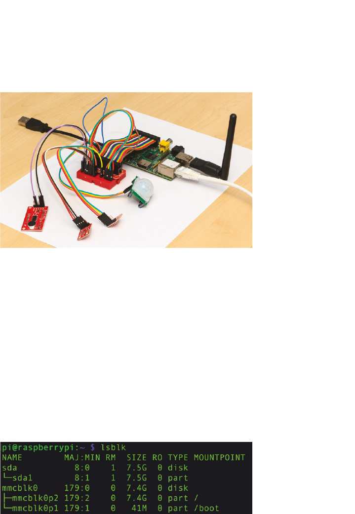
203
A more complex output device might be a printer, connected via USB, which is capable of producing
pages of text and graphics at high-speed. Figure 8.1 shows an indoor environmental sensor node at
the University of Glasgow, with a range of input and output devices aached to a Raspberry Pi.
Figure 8.1: Raspberry Pi sensor node deployed at the University of Glasgow. Photo by Krisan Hentschel.
8.2.1 Inspect your devices
It is possible to inspect some of the devices that are aached to your Raspberry Pi. The lsusb
command will display informaon about devices that are connected to your Pi over USB. Observe that
each device has a unique ID. Also noce that the Ethernet adapter is connected via USB, which is the
reason for slow network performance on Raspberry Pi.
The lsblk command will display informaon about block devices, which are generally, storage
devices, connected to your Pi. Figure 8.2 shows the reported block devices on a Raspberry Pi 3 with
an 8GB SD card. File system mount points for each paron are given. Note that sda1 and mmcblk0
alias to the same physical device. The next chapter covers le systems, presenng a more in-depth
study of block storage facilies in Linux.
Figure 8.2: Typical output from the lsblk command.
8.2.2 Device classes
Look at the /proc/devices le to see devices that are registered on your system. This le shows
that Linux disnguishes between two fundamental classes of devices: character and block devices.
A character device transfers data at byte granularity in arbitrary quanes. Data is accessed as a
stream of bytes, like a le, although it may not be possible to seek to a new posion in the stream.
Chapter 8 | Input/output

Operang Systems Foundaons with Linux on the Raspberry Pi
204
Example character devices include /dev/tty, which is the current interacve terminal and /dev/
watchdog, which is a countdown mer.
A block device transfers data in xed-size chunks called blocks. These large data transfers may
be buered by the OS. A block device supports a le system that can be mounted, as described in
Chapter 9. Example block devices include storage media like a RAM disk or an SD card (which may
be known as /dev/mmcblk0 on your system).
Other classes of device include network devices, which operate on packets of data, generally
exchanged with remote nodes. See Chapter 10 for more details.
8.2.3 Trivial device driver
To present the typical Linux approach to devices, this secon implements a trivial character device
driver. A driver is a kernel module that provides a set of funcons enabling the device to be mapped
to a le abstracon. Once the module is loaded, we can add a device le for it and interact with the
device via the le.
The C code below implements the trivial device driver as a kernel module. This is a character-level
device that returns a string of characters when it is read. In homage to the inimitable Douglas Adams,
our device is called ‘The Meaning of Life,’ and it supplies an innite stream of * characters, which have
decimal value 42 in ASCII or UTF8 encoding.
The key Linux API call is register_chrdev, which allows us to provide a struct of le operaons to
implement interacon with the device. The only operaon we dene is read, which returns the *
characters. The registraon funcon returns an int, which is the numeric idener the Linux kernel
assigns to this device.
We use this idener to ‘aach’ the driver to a device le, via the mknod command. See the bash code
below for full details of how to compile and load the kernel module, aach the driver to a device le,
then read some data.
The stream of characters appears fairly slowly when we cat the device le. This is because our code is
highly inecient; we use the copy_to_user call to transfer a single character at a me from kernel
space to user space.
Lisng 8.2.2: Example device driver C
1 #include <linux/cdev.h>
2 #include <linux/errno.h>
3 #include <linux/fs.h>
4 #include <linux/init.h>
5 #include <linux/kernel.h>
6 #include <linux/module.h>
7 #include <linux/uaccess.h>
8
9 MODULE_LICENSE("GPL");
10 MODULE_DESCRIPTION("Example char device driver");
11 MODULE_VERSION("0.42");

205
12
13 static const char *fortytwo = "*";
14
15 static ssize_t device_le_read(structle*le_ptr,
16 char__user*user_buer,
17 size_t count,
18 lo_t*position){
19 int i = count;
20 while (i--)
21 if(copy_to_user(user_buer,fortytwo,1)!=0)
22 return -EFAULT;
23 return count;
24 }
25
26 static structle_operationsdriver_fops={
27 .owner = THIS_MODULE,
28 .read =device_le_read,
29 };
30
31 static intdevice_le_major_number=0;
32 static const char device_name[] = "The-Meaning-Of-Life";
33
34 static int register_device(void) {
35 int result = 0;
36 result = register_chrdev(0, device_name, &driver_fops);
37 if( result < 0 ) {
38 printk(KERN_WARNING "The-Meaning-Of-Life: "
39 "unable to register character device, error code %i", result);
40 return result;
41 }
42 device_le_major_number=result;
43 return 0;
44 }
45
46 static void unregister_device(void) {
47 if(device_le_major_number!=0)
48 unregister_chrdev(device_le_major_number,device_name);
49 }
50
51 static int simple_driver_init(void) {
52 int result = register_device();
53 return result;
54 }
55
56 static void simple_driver_exit(void) {
57 unregister_device();
58 }
59
60 module_init(simple_driver_init);
61 module_exit(simple_driver_exit);
Lisng 8.2.3: Using the new device Bash
1 sudo make -C /lib/modules/`uname -r`/build M=`pwd` modules
2 sudoinsmodmeaningoife.ko
3 DEVNUM=`cat /proc/devices | grep Meaning | cut -d' ' -f 1`
4 sudo mknod /dev/meaning c $DEVNUM 0
5 cat /dev/meaning
6 ^C
Chapter 8 | Input/output
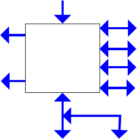
Operang Systems Foundaons with Linux on the Raspberry Pi
206
8.3 Connecng devices
8.3.1 Bus architecture
Since the Raspberry Pi is built around a commercial system-on-chip soluon, which is also used
for mobile phone devices, it has a rich set of direct IO connecons. Figure 8.3 presents this IO
connecvity at an abstract level.
Some connecons are point-to-point, such as the UART (universal asynchronous transmier/receiver)
for direct device to device communicaon. Others allow mulple devices to share a bus, i.e., signals
travel along shared wires and are directed to the appropriate device. The I
2
C bus supports over 1000
devices; these share data, clock and power wires, with each device having a unique address to direct
message packets.
Some IO interfaces are principally for output, such as HDMI for video output to screen. Other
interfaces are for input, such as the CSI (Camera Serial Interface) for digital cameras. Many interfaces,
like the Ethernet network connecon, are bidireconal in that they support both input and output.
Generally, IO is encoded as digital signals. A small number of interfaces use analog signals, such as
the audio-out port. The GPIO signals are all digital; unlike Arduino devices, the Raspberry Pi does not
include a built-in analog-to-digital converter.
Figure 8.3: IO architectural diagram for Raspberry Pi.
In terms of bandwidth, low bandwidth connecons (like those on the right-hand side of SoC in
Figure 8.3) operate around 10kbps. High bandwidth connecons (like those at the boom of SoC
in Figure 8.3) operate around 100Mbps. One peculiarity of the Raspberry Pi architecture is that the
ethernet piggybacks onto the USB interface, which somemes restricts network bandwidth.
More convenonal, larger computers may have higher performance buses such as PCI Express. These
are useful for powerful devices such as graphics cards that need to process and transfer bulk data
extremely rapidly.
i
i
“chapter” — 2019/8/13 — 21:04 — page 3 — #3
i
i
i
i
i
i
Raspberry Pi
System-on-Chip
USB
Ethernet
Video out
Audio out
UART (serial comms)
SPI
I
2
C
GPIO
Camera serial interface

207
8.4 Communicang with Devices
8.4.1 Device Abstracons
From user space, devices generally appear like les, and processes interact with devices using standard
le API calls like open and read. Some devices support special commands, accessed using the generic
ioctl system call on Linux. We use ioctl for device-specic commands that cannot be mapped
easily onto the le API.
A simple example involves the console. It is possible to set the status LEDs for an aached keyboard
using ioctl calls. The Python script below ashes the scroll lock on then o for two seconds. Try this on
your Raspberry Pi with a USB keyboard aached.
Lisng 8.4.1: Flash Keyboard LEDs with ioctl Python
1 import fcntl
2 import os
3 import time
4
5 KDSETLED = 0x4b32
6 SCROLL_LED = 0x01
7 NUMLK_LED = 0x02
8 CAPSLK_LED = 0x04
9 RESET_ALL = 0x08
10
11 console_fd = os.open('/dev/console', os.O_NOCTTY)
12 fcntl.ioctl(console_fd, KDSETLED, SCROLL_LED)
13 time.sleep(2)
14 fcntl.ioctl(console_fd, KDSETLED, 0)
15 time.sleep(2)
16 fcntl.ioctl(console_fd, KDSETLED, RESET_ALL)
From kernel space in Linux on Arm, devices are memory-mapped. The kernel device handling code
writes to memory addresses to issue commands to devices and uses memory accesses to transfer data
between device and machine memory.
8.4.2 Blocking versus non-blocking IO
From user space, when you issue an IO command, it may return immediately (non-blocking), or it may
wait (blocking) unl the operaon completes when all the data is transferred. The key problem with
blocking is that IO can be slow, so waing for IO to complete may take a long me. The thread that
iniated the blocking IO is unable to do any other useful work while it is waing.
On the other hand, a non-blocking IO call returns immediately, performing as much data transfer as is
currently possible with the specied device. If no data transfer can be performed, an error status code
is returned.
In terms of Unix le descriptor ags, the O_NONBLOCK ag indicates that an open le should support
non-blocking IO calls. We illustrate this in the source code below, by reading bytes from the /dev/
random device. This device generates cryptographically secure random noise, seeded by interacons
with the outside world such as human interface events and network package arrival mes.
Chapter 8 | Input/output

Operang Systems Foundaons with Linux on the Raspberry Pi
208
If there is insucient entropy in the system, then reads to /dev/random can block waing for more
random interacons to occur. Execute the Python script shown below for several mes; see how long
it takes to complete. You might be able to speed up execuon by moving and clicking your USB mouse
if it is connected to your Raspberry Pi.
Lisng 8.4.2: Reading data from /dev/random Python
1 import os
2
3 r = os.open('/dev/random', os.O_RDONLY)
4 x = os.read(r, 100)
5 print('read %d bytes' % len(x))
6 if len(x) > 0:
7 print(ord(x[len(x)-1]))
The script drains randomness from the system; we top up the randomness with user events like mouse
movement. When there is lile randomness, the call to read blocks, waing for data from/dev/random.
Now modify the Python script to make read operaons to be non-blocking. Do this by changing the
ags in the open call to be os.O_RDONLY | os.O_NONBLOCK. When we execute the script again,
it always returns immediately. If there is no random data available, then it reports an OSError.
8.4.3 Managing IO interacons
There are three general approaches to interacng with IO devices, in terms of structuring a
‘conversaon’ or communicaon session:
1. Polling;
2. Interrupts;
3. Direct memory access (DMA).
The parcular approach is generally implemented at device driver level; it is not directly visible to the
end-user. Rather, the approach is a design decision made by the manufacturer of the hardware device
in collaboraon with the developer of the soware driver.
Subsequent paragraphs explain the three mechanisms and their relave merits. The idea is that a
device has the informaon we want to fetch into memory, and we need to manage this data transfer.
(Alternavely, the device may require the informaon we have in memory, and we need to handle this
transfer.)
The cartoon illustraon in Figure 8.4 presents an analogy to compare the dierent approaches. The
customer (on the le-hand side) is like a CPU requesng data; the delivery depot (on the right-hand
side) is like a device; the package delivery is like the data transfer from device to CPU. In each of the
three cases, this transfer is coordinated dierently.
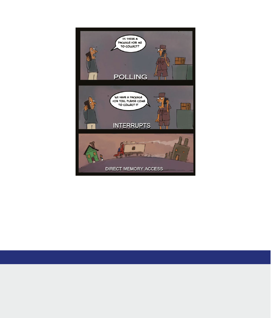
209
Figure 8.4: Parcel delivery analogy for IO transfer mechanisms. Image owned by the author.
Polling
Device polling is acve querying of the hardware status by the client process, i.e., the device driver.
This is used for low-level interacons with simple hardware. Generally, there is a device status ag or
word and the process connually fetches this status data in a busy/wait loop. The pseudo-code below
demonstrates the polling mechanism.
Lisng 8.4.3: Typical device polling code C
1 while (num_bytes) {
2 while (device_not_ready())
3 busy_wait();
4 if (device_ready()) {
5 transfer_byte_of_data();
6 num_bytes--;
7 }
8 }
Soware support for polling is straighorward, as outlined above. It is also easy to implement the
appropriate hardware. However, polling may be inecient in terms of wasted CPU cycles during the
busy/wait loops, parcularly when there is a signicant disparity in speed between CPU and device.
Interrupts
Imagine your phone is ringing right now. You stop reading this book to answer the call. You have been
interrupted! That’s precisely how IO interrupts work. Normal process execuon is temporarily paused,
and the system deals with the IO event before resuming the task that was interrupted.
Chapter 8 | Input/output
Operang Systems Foundaons with Linux on the Raspberry Pi
210
Interrupt handlers are like system event handlers. A handler roune may be registered for a parcular
interrupt. When the interrupt occurs (physically, when a pin on the processor goes high) the system
changes mode and vectors to the interrupt handler.
Secon 8.5 explains the details regarding how to dene and install an interrupt handler in Linux. This
is probably the most common way to deal with IO device interacon.
Direct memory access
The movaon underlying direct memory access (DMA) is to minimize processor involvement in IO
data transfer. For polling and interrupts (collecvely known as programmed IO) the processor explicitly
receives each word of data from the device and writes it to a local memory buer, or vice versa for
data transfer to the device.
With DMA, the processor merely iniates the transfer of a large block of memory, then receives
a nocaon (via an interrupt) when the enre transfer is completed. This reduces context switching
overhead from being linear in the data transfer size to a small, constant cost.
The key complexity of DMA is that the hardware device must be much more intelligent since it needs
to interface directly with the memory controller to copy data into the relevant buer. DMA is most
useful for high-bandwidth devices such as GPUs and hard disk controllers, not for smaller-scale
embedded systems.
The Raspberry Pi has 16 DMA channels, which may be used for high-bandwidth access to IO
peripherals. Various open-source libraries exploit this facility.
8.5 Interrupt handlers
There are three kinds of events that are managed by the OS using the handler paern. These are:
1. Hardware interrupts, which are triggered by external devices.
2. Processor excepons, which occur when undened operaons (like divide-by-zero) are executed.
3. Soware interrupts, which take place when user code issues a Linux system call, encoded as an Arm
SWI instrucon.
This secon focuses on hardware interrupts, but the mechanisms are similar for all three kinds of events.
Interrupt-driven IO can be more ecient than polling, given relave speed disparity between
processor and IO device. A context switch occurs (from user mode to kernel mode) only when an
interrupt is generated, indicang there is IO acvity to be serviced by the processor. There is minimal
busy-waing with interrupts. Figure 8.5 presents a sequence diagram to show the interacons
between CPU and device for interrupt-driven programmed IO.
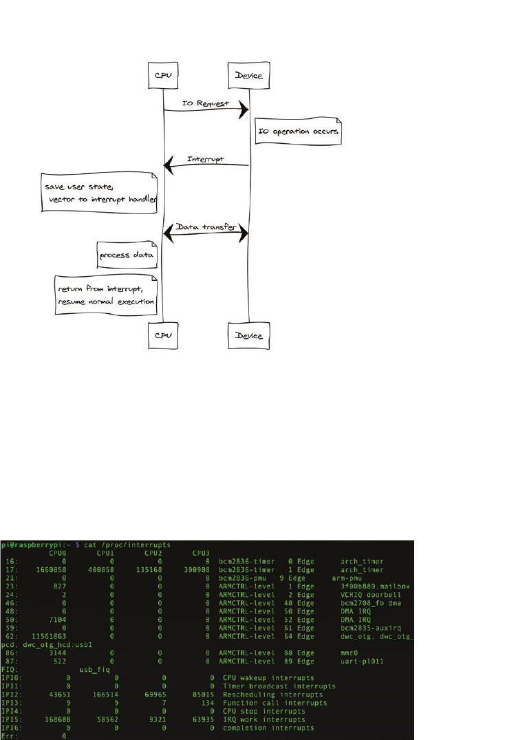
211
Figure 8.5: Sequence Diagram to show communicaon between CPU and Device during Interrupt-Driven IO.
8.5.1 Specic interrupt handling details
Look at the /proc/interrupts le on your Raspberry Pi. This lists the stascs for how many
interrupts have been seen by the system. Figure 8.6 shows an example from a Raspberry Pi 2 Model
B that has been running for several hours. Each interrupt has an integer idener (le-most column),
a count of how many mes it has been handled by CPU0 (second le column) and other CPUs (in
subsequent columns), and a name for the event that device that triggered the interrupt (right-most
column). The timer and dwc_otg devices are likely to have the highest interrupt counts.
Figure 8.6: Sample /proc/interrupts le.
Interrupt handlers, also known as interrupt service rounes, are generally registered during system
boot me, or when a module is dynamically loaded into the kernel. An interrupt handler is registered
with the request_irq() funcon, from include/linux/interrupt.h. Required parameters
include the interrupt number, the handler funcon, and the associated device name. An interrupt
handler is unregistered with the free_irq() funcon.
Chapter 8 | Input/output

Operang Systems Foundaons with Linux on the Raspberry Pi
212
In a mul-processor system, interrupt handlers should be registered for all processors, and
interrupts should be distributed evenly. Check /proc/interrupts to verify this if you have
a mulcore Raspberry Pi board.
It is conceivable that, while the system is servicing one interrupt, another interrupt may arrive
concurrently. Some interrupt handlers may be interrupted, i.e., they are re-entrant. Others may not be
interrupted. It is possible to disable interrupts while an interrupt handler is execung, using a funcon
like local_irq_disable() to prevent cascading interrupon.
8.5.2 Install an interrupt handler
The C code below implements a trivial interrupt handler for USB interrupt events. This is a shared
interrupt line, so mulple handlers may be registered for the same interrupt id. Check the /proc/
interrupts le to idenfy the appropriate integer interrupt number on your Pi, and modify the
source code INTERRUPT_ID denion accordingly.
Lisng 8.5.1: Trivial interrupt handler C
1 /* ih.c */
2
3 #include <linux/interrupt.h>
4 #include <linux/module.h>
5
6 MODULE_LICENSE("GPL");
7 MODULE_DESCRIPTION("Example interrupt handler");
8 MODULE_VERSION("0.01");
9
10 #dene INTERRUPT_ID 62 /* this is dwc_otg interrupt id on my pi */
11
12 static int count = 0; /* interrupt count */
13 static char* dev = "unique name";
14
15 static irqreturn_t custom_interrupt(int irq, void *dev_id) {
16 if (count++%100==0)
17 printk("My custom interrupt handler called");
18 return IRQ_HANDLED;
19 }
20
21 static int simple_driver_init(void) {
22 int result = 0;
23 result = request_irq(INTERRUPT_ID, custom_interrupt, IRQF_SHARED,
24 "custom-handler", (void *)&dev);
25 if (result < 0) {
26 printk(KERN_ERR "Custom handler: cannot register IRQ %d\n", INTERRUPT_ID);
27 return -EIO;
28 }
29 return result;
30 }
31
32 static void simple_driver_exit(void) {
33 free_irq(INTERRUPT_ID, (void *)&dev);
34 }
35
36 module_init(simple_driver_init);
37 module_exit(simple_driver_exit);

213
Compile this module as ih.ko, then install it with sudo insmod ih.ko. Then check dmesg to see
whether the module installed successfully and whether custom interrupt handler messages are being
reported in the kernel log. You can also look at /proc/interrupts to see whether your handler is
registered against the appropriate interrupt. Finally, execute sudo rmmod ih to uninstall the module.
A useful ‘real’ interrupt handler example is in linux/drivers/char/sysrq.c, which handles the
magic SysRq key combinaons to recover from Linux system freezes. This code is well worth a careful
inspecon.
8.6 Ecient IO
One of the issues that makes IO slow is the constant need for context switches. When IO occurs, kernel-
level acvity must take place. User-invoked system calls will vector into the kernel, so too do interrupts
generated by the hardware. Switching into the kernel takes me, switching processor mode and saving
user context. DMA minimizes kernel intervenons in IO, which is why it is so much more ecient.
Another ineciency in IO is excessive memory copying. Recall from our simple device driver example
that we used the copy_to_user funcon call, to transfer data from kernel memory to user memory.
The problem is that user code cannot access data stored in kernel memory.
The technique of buering improves performance. The objecve is to batch small units of data into
a larger unit and process this in bulk. Buering quanzes data processing. Eecvely, a buer is a
temporary storage locaon for data being transferred from one place to another.
The technique of spooling is useful for contended resources. A spool is like a queue; jobs wait in the
queue unl they are ready. The canonical example is the printer spooler, but the technique also applies
to other slow peripheral devices. There may be mulple producers and a single consumer, with the
producers wring each job to the spooler much faster than the consumer can perform that job. These
techniques are used to accelerate IO by avoiding the need for processes to wait for slow IO devices.
8.7 Further reading
For a user-friendly introducon to interfacing devices with your Raspberry Pi, check out Molloy’s highly
praccal textbook [1] with its companion website. There are lots of ideas for simple projects involving
small-scale hardware components, building up to a Linux kernel module implementaon task.
The Linux Device Drivers textbook from O’Reilly presents a comprehensive view of IO and the Linux
approach to device drivers [2]. The book is available online for free. Although it is fairly old, dealing
with Linux kernel version 2.6, the concept coverage is wide-ranging and sll highly relevant.
8.8 Exercises and quesons
8.8.1 How many interrupts?
Produce a simple script that parses the /proc/interrupts le and monitor the number of interrupts per
second. Why might it be sensible to check the le at minute intervals and divide by 60 to get the per-
second interrupt rate?
Chapter 8 | Input/output

Operang Systems Foundaons with Linux on the Raspberry Pi
214
8.8.2 Comparave complexity
Draw a table with the following rows and columns:
Fill in this table for the following devices, esmang the relave costs and complexies for each device:
1. USB mouse;
2. Depth-sensing USB camera;
3. SATA disk controller;
4. Scrolling LED text display screen.
8.8.3 Roll your own Interrupt Handler
Develop a more interesng interrupt handler, based on the trivial example in Secon 8.5.2. See
whether you can write a handler for a dierent interrupt event. Search online for helpful tutorials.
8.8.4 Morse Code LED Device
Imagine an LED that has a character device driver in Linux, so that when you write characters to the
device, the LED ashes the corresponding leers in Morse code.
You could choose to use your scroll lock key or Pi on-board status LED, as outlined in this chapter.
Alternavely, you might aach an external LED component to the GPIO pins.
You will need to implement a device driver with a denion for the write funcon, but you could use
the trivial character device driver from Secon 8.2.3 as a template. You want the rate of Morse code
ashing to be readable, but it would be nice to allow the write operaons to return while the Morse
code message is being (slowly) broadcast. What would you do if another write request occurs while
the rst message is sll in progress?
low / med / high
Device driver implementaon complexity.
Device hardware complexity.
Typical device cost.
Typical device speed.

215
References
[1] D. Molloy, Exploring Raspberry Pi: Interfacing to the Real World with Embedded Linux. Wiley, 2016.
[2] J. Corbet, A. Rubini, and G. Kroah-Hartman, Linux Device Drivers, 3rd ed. O’Reilly, 2005,
hps://www.oreilly.com/openbook/linuxdrive3/book/
Chapter 8 | Input/output

Chapter 9
Persistent storage
Operang Systems Foundaons with Linux on the Raspberry Pi
218
9.1 Overview
Where does data go when your machine is powered down? Volale data, stored in RAM, will be lost;
however, data saved on persistent storage media is retained for future execuon. A le system is a key OS
component that supports the consolidaon of persistent data into discrete, manageable units called les.
The Linux design philosophy is oen summarized as, ‘Everything is a le.’ All kinds of OS enes,
including processes, devices, pipes, and sockets, may be treated as les. For this reason, it is important
to have a good understanding of the Linux le system since it underpins the enre OS.
What you will learn
Aer you have studied the material in this chapter, you will be able to:
1. Illustrate the directed acyclic graph nature of the Linux le system.
2. Appreciate how the user-visible le system maps onto OS-level le system concepts and primives.
3. Explain how le system directories work, to index and locate le contents.
4. Analyze the trade-os involved in dierent le system design decisions, with reference to parcular
implementaons such as FAT and ext4.
5. Understand the need for le system consistency and integrity, idenfying approaches to preserve
or repair this integrity.
6. Idenfy appropriate techniques for le system operaons on a range of modern persistent storage
media.
9.2 User perspecve on the le system
9.2.1 What is a le?
A le is a collecon of data that is logically related; it somehow ‘belongs’ together. A le is a ne-
grained container for data; conceptually, it is the smallest discrete unit of data in a le system. Regular
les may contain textual data (read with ulies like cat or less) or binary data (read with ulies
like hexdump or strings). The le command will report details about a single le. It uses the built-in
stat le system call to determine basic informaon about the target le, and then it checks a set of
‘magic’ heuriscs to guess the actual type of the le based on its contents.
Other ulies infer the type of a le from its extension (the leers aer the dot in the lename).
However, this is not always a reliable guide to the le type, since the extension is simply a part of the
lename and can be modied by users.
In Linux, everything is a le (at least, everything appears to be a le). In simplest terms, this means
everything is addressable via a name in the le system, and these names can be the target of le
system calls such as stat. Enes that aren’t actually regular les have disnct types. For instance,
if you execute ls -l in a directory, you will see the rst character on each line species the disnct
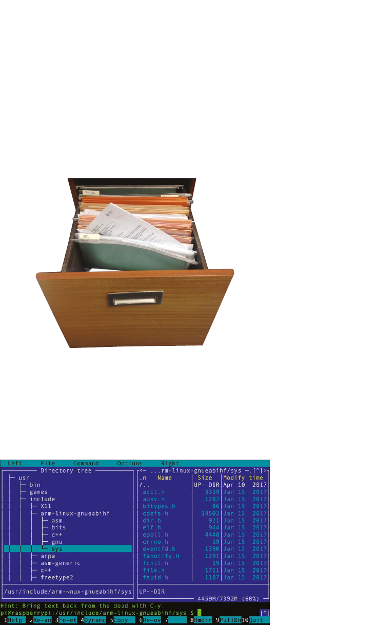
219
type. For directories, this is d, for character devices, it is c, and for symbolic links it is l. The full set of
types is specied in /usr/include/arm-linux/sys/stat.h — look at this header le and search
for Testmacrosforletypes.
9.2.2 How are mulple les organized?
Collecons of les can be grouped together into directories, somemes called folders. A directory contains
les, including other directories. The le system abstracon is a skeuomorphism, designed to resemble
the familiar paper ling cabinet, as shown in Figure 9.1. Each le corresponds to a paper document;
a directory corresponds to a card folder; the enre le system corresponds to the ling cabinet.
Figure 9.1: Tradional ling cabinet containing folders with paper documents. Photo by author.
Linux has a single, top-level root directory, denoted as /, which is the ancestor directory of all other
elements in the le system. We might assume this rooted, hierarchical arrangement leads to a
tree-based structure, and this is oen the graphical depicon of the hierarchy, e.g., in the Midnight
Commander le manager layout shown in Figure 9.2.
Figure 9.2: Midnight commander le manager shows a directory hierarchy as a tree.
Chapter 9 | Persistent storage
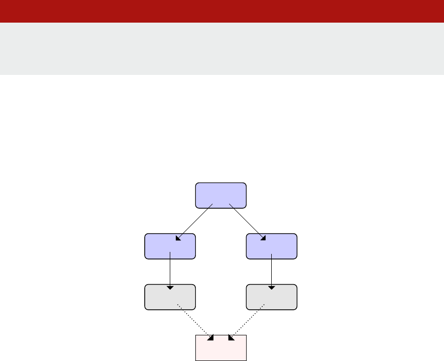
Operang Systems Foundaons with Linux on the Raspberry Pi
220
However, les can belong to mulple directories due to hard links. For example, consider this sequence
of commands:
Lisng 9.2.1: File creaon example Bash
1 cd /tmp
2 mkdir a; mkdir b
3 echohello>a/thele.txt
4 lna/thele.txtb/samele.txt
where /tmp/a/thele.txt and /tmp/b/samele.txt are actually the same le. Try eding one of them,
and then viewing the other. You will observe that the changes are carried over; also that the two
lenames have common metadata when viewed with ls -l. Maybe lenames should be considered
more like pointers to les, rather than the actual le themselves. This leads to a graph-like structure,
see Figure 9.3. However, if you try to remove one of the les, e.g., rm/tmp/a/thele.txt, then the
link is removed, but the le is sll present. It can be accessed via the other link.
Figure 9.3: Graphical view of mulple linked les that map to the same underlying data.
Note that les can belong to mulple directories, (i.e., have mulple hard links) but directories cannot
have extra links. For example, try to do ln /tmp/a /tmp/b/another_a and noce the error that
occurs. Addional hard links for directories are not allowed. This is because we want to prevent cycles
into the directory hierarchy. If we consider a link to be a directed edge in the directory graph, then we
want to enforce a directed acyclic graph. If the only nodes that can have mulple incoming edges are
regular les (i.e., nodes with no successors), then it is impossible to introduce cycles into the graph.
Directory cycles are undesirable since they make it more complex to traverse the directory hierarchy.
Also, it is possible to create cycles of ‘garbage’ directories that are unreachable from the root directory.
There is a further restricon on hard links created with the ln command: such links cannot span
across dierent devices. Although Linux presents the abstracon of a unied directory namespace
with a single root directory, actually mulple devices (disks and parons) may be incorporated into
i
i
“chapter” — 2019/8/13 — 20:50 — page 3 — #3
i
i
i
i
i
i
/tmp
a
b
thefile.txt samefile.txt
hello

221
this unied namespace. Because of the way in which hard links are encoded (see later secon on
inodes) Linux only supports hard links within a single device.
So links or symbolic links (abbreviated as symlinks) are much more exible. These are textual pointers
to paths in the le system. Use ln -s to set up a symlink. These links can be cyclical and can span
mulple devices, unlike hard links. The key property of symlinks is that they are merely strings, like the
lenames and paths you use for interacve commands on the terminal. The symlink strings are not
veried and may be ‘dangling’ links to non-existent les or directories.
9.3 Operaons on les
There is a standard set of le-related acons that every Unix-derived OS must support, known as the
POSIX library funcons for les and directories.
First, to operate on the data stored in a le, it is necessary to open the le, acquiring a le descriptor
which is an integer idener. The OS maintains a table of open les across the whole system; use the
lsof command to list currently open les.
When we open a le, we state our usage intenons: are we only reading? or wring? or appending to
the end of a le? These intenons are checked against relevant le permissions. The operaon fails,
and an error returned (which the programmer must check) if there is a permission violaon.
This le descriptor should be closed when the process has nished operang on the le data. Too
many open le descriptors can cause problems for OS. There are strict limits imposed on the number
of open les, for performance reasons, to avoid kernel denial-of-service style aacks.
The ulimit -n command will display the open le limit for a single process. On your Raspberry Pi,
this might be set to 1024.
You can check that this limit is enforced with a simple Python script that repeatedly opens les and
retains the le descriptors:
Lisng 9.3.1: Open many les in rapid succession Python
1 i = 0
2 les=[]
3 while True:
4 les.append(open("le"+str(i)+".txt", "w+"))
5 i += 1
Noce this fails before creang 1024 les; some les are already open (such as the Python interpreter
and standard input, output and error streams).
There is also a system-wide open le limit, cat/proc/sys/fs/le-max to inspect this value.
The le /proc/sys/fs/le-nr shows the current number of open les across the whole system.
Chapter 9 | Persistent storage
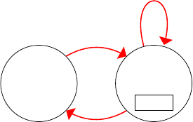
Operang Systems Foundaons with Linux on the Raspberry Pi
222
Once a process has acquired a le descriptor, as a result of a successful open call, it is possible to
operate on that le’s data content. This may involve reading data from or wring data to the le.
There is the implicit noon of a posion within a le, tracking where the pointer associated with the
le descriptor is ‘at.’ The pointer is implicitly at the beginning of the le with open (unless we specify
append mode when it starts at the end). As we read and write bytes of data, we advance the pointer.
We can reset the pointer to an arbitrary posion in the le with the lseek call. It is also possible to
change the size of an open le with the truncate call. Figure 9.4 shows the state transions of a le
descriptor as these calls occur.
Figure 9.4: State machine diagram showing sequence of le system calls (in red) for a single le.
File metadata updates, such as name, ownership, and permissions, are atomic. There is no need to
open the le for these operaons; le system calls simply use the name of the le.
9.4 Operaons on directories
Although directories appear to be like les, they are opened with a disnct API call opendir, to allow
a program to iterate through the directory contents.
Directory modicaon operaons are atomic, from the programmer perspecve. Operaons like
moving, copying, or deleng les have le system API calls, but these require string lename paths
rather than open le descriptors. Note that all the standard bash le manipulaon commands like mv
and rm have API equivalents for programmac use.
In the same way, metadata updates can be performed programmacally, and appear to be atomic.
Again, these operaons require string lename paths.
9.5 Keeping track of open les
For each process, the Linux kernel maintains a table to track les that have been opened by that
process. The integer le descriptor associated with the open le, also known as a handle, corresponds
to an index into this per-process table. The table is called les_struct, dened in include/
linux/fdtable.h; it is a eld of the task_struct process control block.
Each entry in the les_struct table has a pointer to a structle object, which is dened in
include/linux/fs.h. These objects reside in the system-wide le table, dened in fs/le_
i
i
“chapter” — 2019/8/13 — 20:50 — page 4 — #4
i
i
i
i
i
i
closed
opened
pos=X
open
close
read/write/lseek/ ...
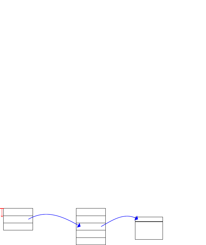
223
table.c. The structle data structure maintains the current le posion within the open le,
the permissions for accessing the le, and a pointer to a dentry object.
The dentry (short for ‘directory entry’) encodes the lename in the directory hierarchy and links the
name with the locaon of the le on a device, represented as an inode (see Secon 9.10). This data
structure is dened in include/linux/dcache.h.
A single process may have mulple le descriptors, corresponding to mulple entries in the
les_struct table, that point to the same system-wide structle object. This is possible with
the dup system call that creates a fresh copy of a le descriptor.
Mulple processes may have their own disnct le descriptors, in their own les_struct table, that
point to the same system-wide structle object. This is possible because the per-process state is
cloned when a new process is forked, so the forked process will inherit open le descriptors from its
parent process.
In both the above situaons, there is a single le oset. This means that if the le oset is modied via
one of the aliased le descriptors, then the oset is also changed for the other(s).
It is also possible that dierent entries in the system-wide le table might point to the same directory
entry. This happens if mulple processes open the same le, or even if a single process opens the
same le several mes. In these cases, each disnct structle has its own associated le oset.
Figure 9.5: Open les are tracked in a per-process le table (le), which contains pointers into the system-wide le table (center), which references
directory locaon informaon to access the underlying le contents.
9.6 Concurrent access to les
The previous secon introduced the noon of mulple processes accessing the same open le.
In general, mulple readers are straighorward. If each reading process has a disnct le descriptor
mapping onto a disnct structle, then each reader has its own unique posion in the le.
Although Linux permits concurrent wring processes, there may be problems and inconsistencies.
If a le is opened with the O_APPEND ag set, then the OS guarantees that writes will always safely
append even with mulple writers. The issue here is that, while the two processes may append their
writes to the le in the correct order, this data may be interleaved between the processes.
i
i
“chapter” — 2019/8/13 — 20:50 — page 5 — #5
i
i
i
i
i
i
file descriptor
offset
per-process
files_struct
table
table of
struct file
objects
fget(int fd)
dentry
+filename
+parent
+location
f_path.dentry
Chapter 9 | Persistent storage

Operang Systems Foundaons with Linux on the Raspberry Pi
224
It is possible to lock a le to prevent concurrent access by mulple processes. There are various ways
to perform le-based locking. The C code below demonstrates the use of lockf, which relies on the
underlying fcntl system call.
Lisng 9.6.1: Lock the log.txt le for single writer access C
1 #include <stdio.h>
2 #include <stdlib.h>
3 #include <string.h>
4 #include <sys/le.h>
5 #include <unistd.h>
6
7 /* takes a single integer command-line
8 * parameter, specifying how long to
9 * sleep after each write operation
10 */
11 int main(int argc, char **argv) {
12
13 int t = atoi(argv[1]);
14 int i;
15 char msg[30];
16
17 int fd = open("log.txt", O_WRONLY|O_CREAT|O_APPEND, 0666);
18 if(fd == -1){
19 perror("unabletoopenle");
20 exit(1);
21 }
22 /* lock the open le */
23 if (lockf(fd, F_LOCK, 0) == -1) {
24 perror("unabletolockle");
25 exit(1);
26 }
27
28 for (i=0; i<10; i++) {
29 sprintf(msg, "sleeping for %d seconds\n", t);
30 write(fd, msg, strlen(msg));
31 sleep(t);
32 }
33
34 /* unlock le */
35 if (lockf(fd, F_ULOCK, 0) == -1) {
36 perror("unabletounlockle");
37 exit(1);
38 }
39 close(fd);
40 return 0;
41 }
If a parcular le is already locked, then a subsequent call to lockf blocks unl that le has been
unlocked. Try compiling this C code, then running two instances of the executable concurrently to
observe what happens—the rst process should complete all its writes to the log before the second
process is allowed to write anything.
Note that this kind of le-based locking on Linux is only advisory. Processes may ‘ignore’ le locks
enrely and proceed to read from or write to open les without respecng locks.
225
9.7 File metadata
Metadata describes the properes of each le. There is a standard set of aributes that the Linux le
system supports directly, so these items are recorded for all les.
This includes user-centric metadata, such as the textual name and type of the le. The type is
convenonally encoded as part of the name, a sux aer the nal period character in the name.
Parcular le system formats may impose restricons on names, such as their length or permied
characters.
The le name is a human-friendly label for the user to specify the le of interest. However, the le
system maintains a unique numeric idener for each le, which is used internally. It is the case that
mulple names may actually map to the same le (i.e., the same numeric id) in the directed acyclic
graph directory structure of Linux, as explained in Secon 9.2.2.
The size of the le is specied in bytes, i.e., its length. The le occupies some number of blocks on
a device, but these blocks may not be full if the le size is not a precise mulple of the block size.
Unlike null-terminated C-style strings, there is no explicit end-of-le (EOF) marker. Instead, we must
use the length of the le to determine when we reach the end of its data.
File access permissions metadata is supported in Linux. Each le has an owner (generally the creator
of the le, although the chown command can modify the owner). Each le has a group (to which the
owner may or may not belong; note the chgrp command can modify the group). The owner and group
are encoded as integer ideners, which may be looked up in the relevant tables in /etc/passwd
and /etc/group les.
For permissions, there are nine bits of metadata, three each for the owner, the group, and
everyone else. Each triple of bits (from most signicant to least signicant bit) encodes read, write and
execute permission respecvely. Figure 9.6 illustrates these permission bits. This metadata can be set
using the chmod command, followed by three octal numbers for the three triplets. More advanced
capabilies and ne-grained permissions are supported by the SElinux system.
Figure 9.6: The 9-bit permissions bitstring is part of each le’s metadata—in this example, the owner can read and write to the le, all other users can only
read the le.
Timestamp elds record creaon me, most recent edit me, and most recent access me for each
le. These are recorded as seconds since 1970, the start of the Unix epoch. Since they are signed
32-bit integers, the maximum mestamp that can be encoded is some me on 19 January 2038.
i
i
“chapter” — 2019/8/13 — 20:50 — page 6 — #6
i
i
i
i
i
i
user
1 1 0
r w x
group
1 0 0
r w x
other
0 1 0
r w x
Chapter 9 | Persistent storage
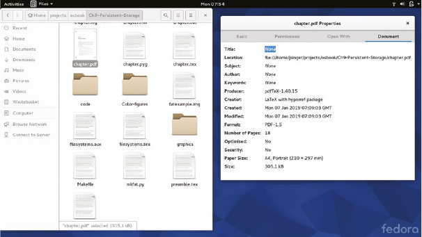
Operang Systems Foundaons with Linux on the Raspberry Pi
226
Recent Linux patches have extended the mestamp elds to 64 bits, with support for nanosecond
granularity and a longer maximum date.
The most important administrave metadata is the actual locaon of the le data on the disk. The precise
details depend on the specic nature of the le system implementaon, which we will cover in later secons.
Somemes extra metadata is supported by graphical le managers like Naulus (for Gnome) or
Dolphin (for KDE). These might include per-le applicaon associaons or graphical icons).
For specic kinds of les, applicaon-specic metadata may be included within the le itself, e.g., MP3 audio
les include id3 tags for arst and tle, PDF les include page counts. While this is not navely supported
within the Linux le system, it might be parsed and rendered by custom le managers, e.g., see Figure 9.7.
Figure 9.7: Naulus le manager parses and displays custom metadata for a PDF le.
9.8 Block-structured storage
A le system is an abstracon built on top of a secondary storage facility such as a hard disk or,
on a Raspberry Pi, an SD card.
Typical le systems depend on persistent, block-structured, random access storage.
Persistent means the data is preserved when the machine is powered o.
Block-structured means the storage is divided into xed-size units, known as blocks. Each block may
be accessed via a unique logical block address (LBA).
Random access means the blocks may be accessed in any order, as opposed to constraining access
to a xed sequenal order (which would be the case for magnec tape storage, for instance).
While magnec hard disks have physical geometries, and data is stored in locaons based on tracks
(circular strips on the disk) and sectors (sub-divisions of tracks), more recent storage media such as
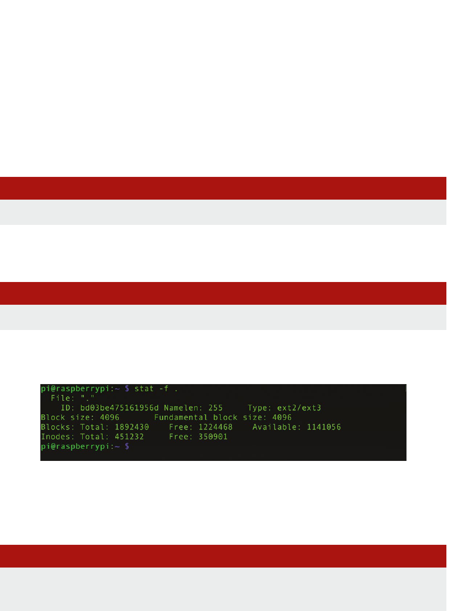
227
solid-state storage do not replicate these layouts. In this presentaon, we will deal in terms of logical
blocks; which is an abstracon that can be supported by all modern storage media.
So, a storage device consists of idencally sized blocks, each with a logical address. This is similar
to pages in RAM (see Chapter 6) only blocks are persistent. Oen the block size is the same as the
memory page size, to facilitate ecient in-memory caching of disk accesses.
We can examine the block size and the number of blocks for the Raspbian OS image installed on your
Raspberry Pi SD card. In a terminal, type
Lisng 9.8.1: Simple stat command Bash
1 stat -fc %s /
to show the block size (in bytes) of your le system. This should be 4096, i.e., 4KB. To see the details
of free and used blocks in your le system, type
Lisng 9.8.2: Another simple stat command Bash
1 stat -f /
and you should get a data dump like that shown in Figure 9.8. This displays the space occupied by
metadata (the inodes) and by actual le data (the data blocks).
Figure 9.8: Output from the stat command, showing le system block usage.
A block is the smallest granular unit of storage that can be allocated to a le. So a le containing just
10 bytes of data, e.g., hi.txt in the example below, actually occupies 4K on disk.
Lisng 9.8.3: Dierent ways to measure le size Bash
1 echo "hello you!" > hi.txt
2 ls -l hi.txt # shows actual data size
3 du -h hi.txt # shows data block usage
Chapter 9 | Persistent storage
Operang Systems Foundaons with Linux on the Raspberry Pi
228
This wasted space is internal fragmentaon overhead, caused by xed block sizes. The 4K block size
is generally a good trade-o value for general purpose le systems.
This secon has outlined block-structured storage at the device level; we present more details on
devices in the chapter covering IO. Next, we will explore how to build a logical le system on top of
these low-level storage facilies.
9.9 Construcng a logical le system
Given this block-based storage scheme, how do we build a high-level le system on top?
Some blocks must be dedicated to indexing, allowing us to associate block addresses with high-level
les and directories. Other blocks will be used to store user data, the contents of les. As outlined
above, the smallest space a le can occupy is a single block. Depending on the block size and the
average le size, this may cause internal fragmentaon, where space is allocated to a le but unused
by that les.
A le system architect makes decisions about how to arrange sets of blocks for large les. There
are trade-os to consider, such as avoiding space fragmentaon and minimizing le access latency.
Possible strategies include:
Conguous blocks: a large le occupies a single sequence of consecuve blocks. This is ecient
when there is lots of space, but can lead to external fragmentaon problems (i.e., awkwardly sized,
unusable holes) when les are deleted, or les need to grow in size.
Indexed blocks: a large le occupies a set of blocks scaered all over the disk, with an
accompanying index to maintain block ordering. This reduces locality of disk access and requires
a large index overhead (like page tables for virtual memory). However, there are no external
fragmentaon issues.
Linked blocks: a large le is a linked list of blocks, which may be scaered across the disk. There is
no fragmentaon issue and no requirement for a complex index. However, it is now inecient to
access the le contents in anything other than a linear sequence from the beginning.
Every concrete le system format incorporates such design decisions. First, we consider an abstracon
that allows Linux to handle mulple le systems in a scalable way.
9.9.1 Virtual le system
There are many concrete le systems, such as ext4 and FAT, which are reviewed later in this chapter.
These implementaons have radically dierent approaches to organizing persistent data as les on
disks, reecng diverse design decisions. In general, an OS must support a wide range of le systems,
to enable compability and exibility.
The Linux virtual le system (VFS) is a kernel abstracon layer. The key idea is that the VFS denes a
common le system API that all concrete le systems must implement. The VFS acts as a proxy layer,

229
in terms of soware design paerns. All le-related system calls are directed to the VFS, and then it
redirects each call to the appropriate concrete underlying le system.
Linux presents the abstracon of a unied le system, with a single root directory from which all other
les and directories are reachable. In fact, the VFS integrates a number of diverse le systems, which
are incorporated into the unied directory hierarchy at dierent mount points. Inspect /etc/mtab to
see the currently mounted le systems, their concrete le system types, and their locaons within the
unied hierarchy.
The pseudo-le /proc/lesystems maintains a list of le systems that are supported in your Linux
kernel. Note that the nodev ag indicates the le system is not associated with a physical device.
Instead, the pseudo-les on such le systems are synthesized from in-memory data structures,
maintained by the kernel.
A concrete le system is registered with the VFS via the register_lesystem call. The supplied
argument is a le_system_type, which provides a name, a funcon pointer to fetch the superblock
of the le system and a next pointer. All le_system_type instances are organized as a linked list.
The global variable le_systems in fs/lesystems.c points to the head of this linked list.
The superblock, in this context, is an in-memory data structure that contains key le system metadata.
There is one superblock instance corresponding to each mounted device. Some of this data comes
from disk (where there may be a le system block also called the superblock). Other informaon, in
parcular, the vector of funcon pointers named struct super_operations, is populated from
the concrete le system code base directly. See the lisng below for details of the funcon pointers
that will be lled in by le system-specic implementaons.
Lisng 9.9.1: Vector of le system operaons, from include/linux/fs. C
1 struct super_operations {
2 struct inode *(*alloc_inode)(struct super_block *sb);
3 void (*destroy_inode)(struct inode *);
4 void (*dirty_inode) (struct inode *, intags);
5 int (*write_inode) (struct inode *, struct writeback_control *wbc);
6 int (*drop_inode) (struct inode *);
7 void (*evict_inode) (struct inode *);
8 void (*put_super) (struct super_block *);
9 int (*sync_fs)(struct super_block *sb, int wait);
10 int (*freeze_super) (struct super_block *);
11 int (*freeze_fs) (struct super_block *);
12 int (*thaw_super) (struct super_block *);
13 int (*unfreeze_fs) (struct super_block *);
14 int (*statfs) (struct dentry *, struct kstatfs *);
15 int (*remount_fs) (struct super_block *, int *, char *);
16 void (*umount_begin) (struct super_block *);
17 int (*show_options)(structseq_le*,struct dentry *);
18 int (*show_devname)(structseq_le*,struct dentry *);
19 int (*show_path)(structseq_le*,struct dentry *);
20 int (*show_stats)(structseq_le*,struct dentry *);
21 // ...
22 };
Chapter 9 | Persistent storage
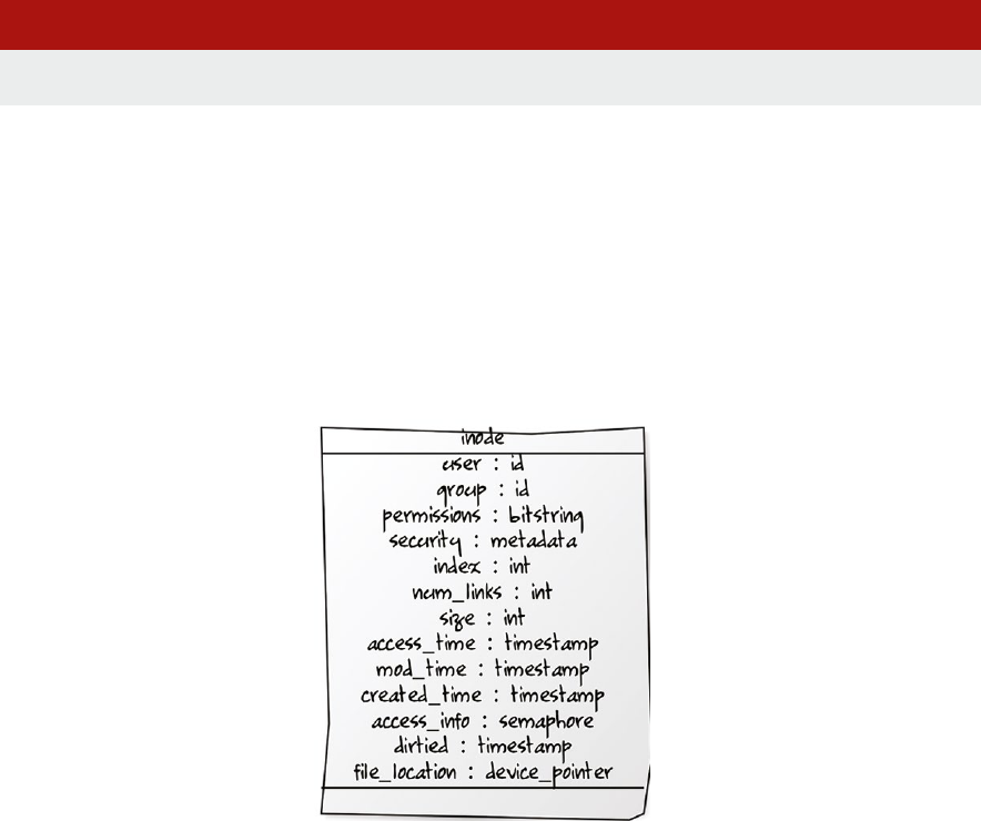
Operang Systems Foundaons with Linux on the Raspberry Pi
230
When a device is mounted, the le system is incorporated into the VFS le hierarchy at the specied
locaon, using locaon specied in the superblock, which is read via the appropriate funcon pointer,
as specied in the named le system’s le_system_type. The mount system call performs this task,
specifying the device to be mounted, the appropriate concrete le system type, and the directory path
at which the le system should be mounted. Try inserng a USB sck in your Raspberry Pi and mounng
it manually. Use strace to trace system call execuon. You may need to disable auto-mounng
temporarily; also use dmesg to nd out the path of the device corresponding to your USB sck.
Lisng 9.9.2: Mounng a USB sck Bash
1 sudo strace mount /dev/sda1 /mnt 2>&1 | grep mount
The superblock handles VFS interacons for an enre le system. Individual les are handled using
structures called inodes and dentries, which are introduced in subsequent secons.
9.10 Inodes
The inode (which stands for index node) is a core data structure that underpins Linux le systems.
There is one inode per enty (e.g., le or directory) in a le system. You can study the denion of
struct inode in the VFS source code at linux/fs.h. A simplied class diagram view of the inode
data structure is shown in Figure 9.9.
Figure 9.9: Class diagram representaon of the inode data structure.
Each inode stores all the metadata associated with a le, including on-device locaon informaon
for the le data. Typical metadata items (e.g., owner identy, le size, and permissions) are stored
directly in the struct. Extended metadata (such as access control lists for enhanced security) are stored
externally, with pointers in the inode structure.

231
As outlined so far, the inode is a VFS-level, in-memory data structure. Other Unix OSs refer to these
structures as vnodes. Concrete le systems may have specialized versions of the inode. For instance,
compare the VFS struct inode denion in include/linux/fs.h with the ext4 variants
struct ext4_inode and struct ext4_inode_info in fs/ext4/ext4.h.
As well as being an in-memory data structure, the inode data is serialized to disk for persistent
storage. Generally, when a nave Linux le system is created, a dedicated conguous poron of the
block storage is reserved for inodes. Each inode is a xed size, so there is a known limit on the number
of inodes (which implies a maximum number of les). Oen the inode table is at the start of the
device. Each inode associated with the device has a unique index number, which refers to its entry in
the inode table. You can inspect the inode number for each le with the ls -i command. Look at the
inode numbers for les in your home directory:
Lisng 9.10.1: Inspecng inode numbers for new les Bash
1 cd ~
2 ls -i
3 echo "hello" > foo
4 echo "hello again" > bar
5 ls -i foo bar
Note the large integer value associated with each le. Generally, newly created les will receive
consecuve inode numbers, as you might be able to see with the newly created foo and bar les
(presuming you do not already have les with these names in your home directory).
9.10.1 Mulple links, single inode
As outlined above, a le name is really just a pointer (a hard link) to an inode. Mulple le names (from
dierent paths in the le system) may map onto the same inode. The num_links eld in the inode
keeps track of how many le names refer to this inode; eecvely this is a reference count.
The reference count is incremented with an ln command and decremented with a corresponding rm
command. When the reference count reaches zero, the inode is orphaned and may be deleted by the
OS, freeing up this slot in the table for fresh metadata associated with a new le.
Note that the inode does not contain links back to the lenames that are associated with this inode.
That info is stored in the directories, separately. The inode simply keeps a count of the number of live
links (valid lenames) that reference it.
9.10.2 Directories
A directory, in abstract terms, is a key/value store or a diconary. It associates le system enty names
(which are strings) onto inode numbers (which are integers). An enty name might refer to a le or a
directory. There is a system-imposed limit on the length of an enty name, which is set to 255 (8-bit)
characters). Use getconf NAME_MAX / to conrm this. If you try to create a le name longer than
this limit, you will fail with a File name too long error.
Chapter 9 | Persistent storage
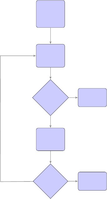
Operang Systems Foundaons with Linux on the Raspberry Pi
232
VFS does not impose a maximum number of entries in a single directory. The only limit on directory
entries is that each entry requires an inode, and there is a xed number of inodes on the le system.
(Use df -i to inspect the number of free inodes, labeled as IFree.)
In every directory, there are two disnguished entries, namely . (pronounced ‘dot’) and ..
(pronounced ‘dot dot’).
. refers to the directory itself, i.e., it is a self-edge in the reference graph. The command cd . is
eecvely a null operaon.
.. refers to the parent directory. The command cd .. allows us to traverse up the directory
hierarchy to the root directory, /. Note that the parent of the root directory is the root directory
itself, i.e., root’s parent is also a self-edge in the reference graph.
Each process has a current working directory (cwd). For instance, you can discover the working
directory of a bash process with the pwd command, or the working directory of an arbitrary process
with PID n by execung the command readlink /proc/n/cwd. Relave path names (i.e., those not
starng with the root directory /) are interpreted relave to the process’s current working directory.
Figure 9.10: Simplied ow chart for Linux directory path lookup, based on code in fs/namei.c
i
i
“chapter” — 2019/8/13 — 20:50 — page 10 — #10
i
i
i
i
i
i
start at
well-known
directory,
e.g. root
or cwd
add info to
nameidata
and update
cache
is this last
element in
path?
extract next
directory
name
from path
exists?
mounted?
accessible?
at end, do
final action,
return
handle
directory
lookup error
yes
no
no
yes
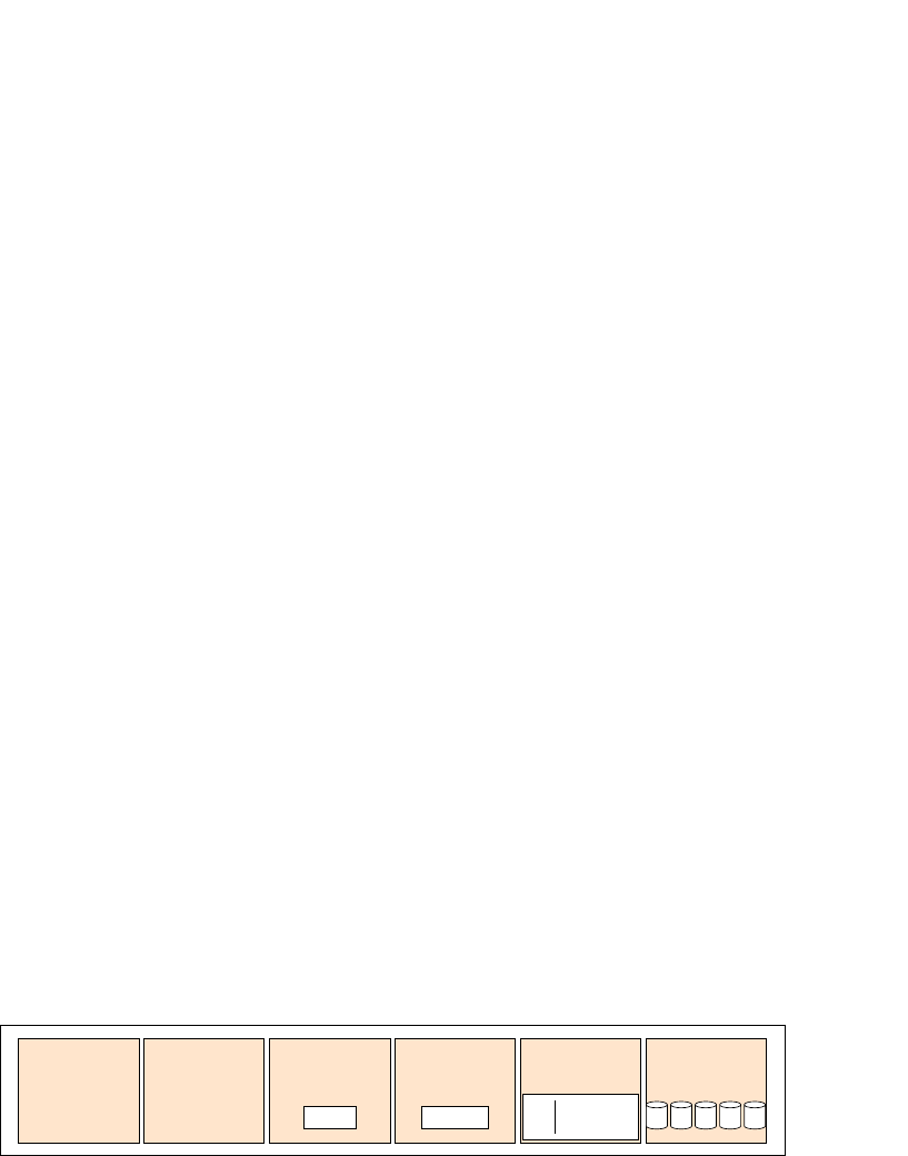
233
Absolute path names (i.e., those starng with the root directory /) are based on a path to a le that
starts from the root directory of the VFS le system. Note that paths may span mulple concrete le
systems since these are mounted at various osets from the VFS root.
One of the key facilies provided by the directory is to map from a lename string to an inode number.
The algorithm presented in Figure 9.10 is a high-level overview of this translaon process. You may
invoke this behavior on the command line by using the namei ulity with a lename string argument.
Translaon of lename strings to inode numbers is an expensive acvity. A data structure called a
directory entry (dentry) stores this mapping. The struct dentry denion is in include/linux/
dcache.h. VFS features a dentry entry cache (dcache) for frequently used translaons. This cache
is described in detail in the kernel documentaon, see Documentation/lesystems/vfs.txt,
along with other VFS structures and mechanisms.
9.11 ext4
The extended le system is the nave le system format for Linux. The current incarnaon is ext4,
although it has much in common with the earlier versions ext2 and ext3.
Look at le /etc/fstab, which shows the le systems that are mounted (i.e., reachable from the
root directory) as part of the OS boot sequence. On your Raspbian system, the default le system is
formaed as ext4 and mounted directly at the root directory.
9.11.1 Layout on disk
The way a le system is laid out on a disk (or a disk paron) is known as its format. For any format,
the rst block is always the boot block. This may contain executable code, in the event that this disk is
used as a boot device. Generally, this boot code sequence is very short and jumps to another locaon
for larger, more complex boong behavior.
Immediately aer the boot block, ext4 has a number of block groups. Each block group is idencal in
size and structure; a single block group is illustrated in Figure 9.11.
Figure 9.11: Schemac diagram showing the structure of an ext4 block group on disk.
The rst two elements of a block group are at xed osets from the start of the block group. The
superblock records high-level le system metadata, such as the overall size of the le system, the size of
each block, number of blocks per block group, device pointers to important areas, and mestamps for
most recent mount and write operaons. The struct ext4_super_block is dened in fs/ext4/
ext4.h. Note the superblock only occupies a single block on disk. This on-disk superblock is disnct
i
i
“chapter” — 2019/8/13 — 20:50 — page 11 — #11
i
i
i
i
i
i
superblock blockgroup
descriptors
data blocks
bitmap
11010
inodes
bitmap
1101100
inode
table
data
blocks
YX Z
1 ext4_inode
2
ext4_inode
...
Chapter 9 | Persistent storage
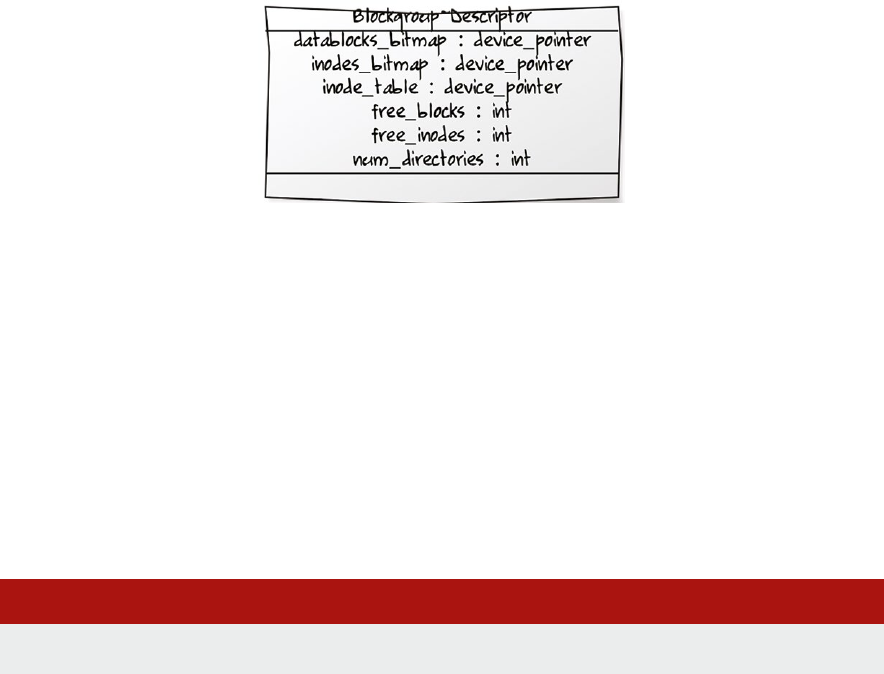
Operang Systems Foundaons with Linux on the Raspberry Pi
234
from the VFS in-memory superblock structure outlined in Secon 9.9.1, although some data is shared
between them.
Ideally, the superblock is duplicated at the start of each block group. This provides redundancy in case
of disk corrupon. If there are many block groups, then the superblock is only sparsely duplicated at
the start of every nth block group.
The block group descriptor table is global; i.e., it covers all blocks. There is one entry in the table for
each block group, which is a struct ext4_group_desc as dened in the ext4.h header. Figure
9.12 presents this data structure as a UML class diagram. Again, the block group descriptor table is
duplicated across mulple block groups for redundancy, like the superblock.
Figure 9.12: Class diagram representaon of a block group descriptor.
All other le system structures are pointed to by the block group descriptor. The block and inode
bitmaps use one bit to denote each data block and inode, respecvely. A bit is set to 1 if the
corresponding enty is used, or 0 if free. These bitmaps may be cached in memory for access speed.
The inode table has one entry, a struct ext4_inode, per le. This table is stacally allocated, as
outlined in Secon 9.10, so there is a xed limit on the number of les. Special inode table entries are
at well-known slots; generally, inode 2 is the root directory for the le system.
The data blocks region of the block group is the largest; these blocks actually store le data content.
Generally, all blocks belonging to a le will be located in a single block group, for the locality.
You can inspect all the details of your ext4 le system on your Raspberry Pi with a command like:
Lisng 9.11.1: Inspect ext4 le system Bash
1 sudo dumpe2fs -h /dev/mmcblk0p2 # for default Raspbian image on SD card
9.11.2 Indexing data blocks
As noted above, there are two dierent data structures for an inode. The generic VFS struct inode
may be converted into a specic ext4_inode with a macro call, EXT4_I(inode).
The key addional informaon is the locaon pointer for the data blocks that comprise the le
content. Actually, an ext4 inode support three dierent techniques for encoding data locaon,
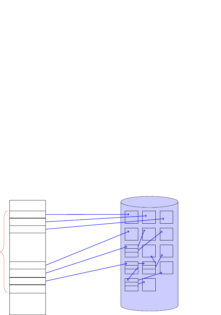
235
unioned over its 60 bytes for physical locaon informaon. Look at fs/ext4/ext4.h and nd the
relevant i_block[EXT4_N_BLOCKS] eld in struct ext4_inode.
The rst approach is direct inline data storage. If the le contents are smaller than 60 bytes, they can
be stored directly in the inode itself. This generally only happens for symlinks with short pathnames,
although it can be used for other short les. (You may need to enable the inline_data feature
when you format the ext4 le system.) This is the only way actual le data is stored in the inode table
secon of the le system.
The second approach is the tradional Unix hierarchical block map structure. This is the same as
in earlier ext2 and ext3 le systems. The 60 bytes of locaon data are split into 15 4-byte pointers
to logical block addresses. The rst 12 pointers are direct pointers to the rst 12 blocks of the le
data. The next pointer is a single indirect pointer; it points to a block containing a table of pointers
to subsequent data blocks for the le. Convenonally, the block size is 4KB, and each pointer is
4B, so it is possible to have 1K pointers in the single indirect block. The next pointer is to a double
indirect pointer, and the nal pointer is to a triple indirect pointer. In total, this allows us to address
over 1 billion blocks, making for a maximum le size of over 4TB. Figure 9.13 illustrates this structure
schemacally, showing pointers for up to the second level of indirecon. Note that the tables of
pointers, for indirect blocks, are stored in data blocks, rather than in the inode table.
Figure 9.13: Schemac diagram of ext4 map indirecon scheme for data block locaons.
This mul-level indirecon scheme has several benets. There are the advantages of direct block
addressing, for short les or the rst few blocks of a long le. There is the advantage of hierarchical
metadata, like mul-level page tables, to avoid wasted space for medium size les. There is the
advantage of indirecon, to avoid bloang inodes directly, for very large les. Check out fs/ext4/
indirect.c for further implementaon details.
i
i
“chapter” — 2019/8/13 — 20:50 — page 13 — #13
i
i
i
i
i
i
direct block 1
direct block 2
direct block 3
direct block 12
...
single indirect
double indirect
triple indirect
15 pointers
(60 bytes)
data data data
data data data
...
data data
...
...
data
...
data
ext4_inode
data blocks
Chapter 9 | Persistent storage
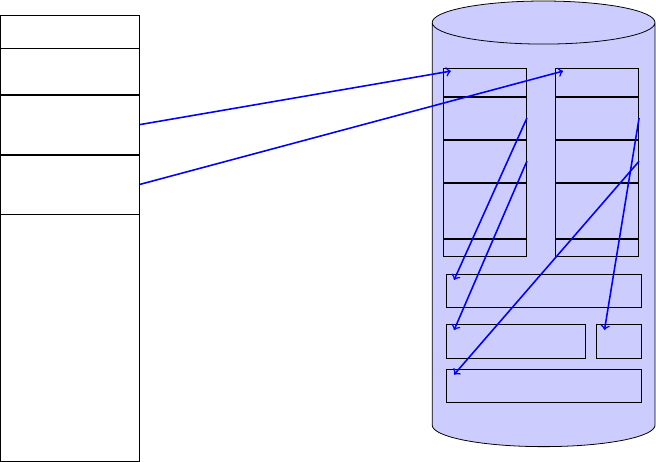
Operang Systems Foundaons with Linux on the Raspberry Pi
236
The third approach, which is new in ext4, involves extents. An extent is a conguous area of storage
reserved for a le (or a part of a le, since a le may consist of mulple extents). An extent is
characterized by a starng block number, a length measured in blocks, then the logical block address
corresponding to the starng block number. See struct ext4_extent in fs/ext4/ext4_
extents.h for details.
The chief benet of an extent-based le system is a reducon in meta-data. Whereas a block
map system requires a metadata entry (a block locaon) for every block, each extent only records
a single logical block address for a conguous run of blocks. It is good pracce to make le data as
conguous as possible, to improve access mes.
The 60 bytes of an ext4_inode may be used to store a 12-byte extent header followed by an array
of up to four 12-byte extent structures.
If there are more than four extents in the le, then the extent data can be arranged as a mul-level
N-ary tree, up to ve levels. Extent data spills out from the inode into data blocks. A data block storing
extent data begins with an ext4_extent_header which states how many extent entries there
are in this block and the tree depth. The entries follow in an array layout. If the tree depth is 0, then
the entries are leaf nodes, i.e., ext4_extent entries poinng directly to extents of data blocks on
disk. If the tree depth is greater than 0, then the entries are index nodes, i.e., ext4_extent_idx
entries, poinng to further blocks of extent data. These structures are all dened in fs/ext4/ext4_
extents.h. Figure 9.14 gives an example, with a two-level extent tree. This is similar to the indirect
block addressing used in the previous approach.
Figure 9.14: Schemac diagram of ext4 extents scheme for data block locaons.
i
i
“chapter” — 2019/8/13 — 20:50 — page 14 — #14
i
i
i
i
i
i
extent_header
n=2, depth=1
extent_index
extent_index
extent_header
n=..., depth=0
extent
extent
...
extent_tail
extent_header
n=...,depth=0
extent
extent
...
extent_tail
data
data data
data
ext4_inode
data blocks

237
9.11.3 Journaling
The ext4 le system supports a journal, a dedicated log le that records each change that is to occur
to the le system. The journal tracks whether a change has started, is in progress, or has completed.
An append-only log le like this is vital when complex le system operaons may be scheduled, which
would cause le system corrupon if they start but do not complete, e.g., due to power failure. The log
may be consulted on system restart to recover the le system to a consistent state, either replaying or
undoing the paral acons.
Transacon records are added to the log rapidly and atomically. The journal le is eecvely a
circular buer, so older entries are overwrien when it lls up. Examine the le /proc/fs/jbd2/
<partition>/info to see stascs about the number of transacon entries in the log.
9.11.4 Checksumming
A checksum is a bit-level error detecon mechanism. This is highly useful for persistent storage, where
there is a possibility of data corrupon.
The most popular algorithm is CRC32c, which generates a 32-bit checksum for an arbitrary size input
byte array. The CRC32c algorithm may be implemented eciently in soware, although some Arm
CPUs have a built-in instrucon to perform the calculaon directly.
The ext4 le system supports CRC32c checksums for metadata. Try the following grep command to
explore elds that have checksums aached:
Lisng 9.11.2: Find checksum elds Bash
1 cd linux/fs/ext4/
2 grep crc *.h
Some checksums are embedded in top-level le system metadata. These include checksum elds in the
superblock and the block group descriptor, although each 32-bit value may be split across two 16-bit
elds in these structures. Checksums are ideal when there are redundant copies of such metadata.
If superblock corrupon is detected, then the metadata can easily be restored by cloning a reserve copy.
Each block group bitmap that tracks free inodes or data blocks also has a checksum to ensure its
integrity. Further, there are checksums for individual le metadata. Each inode has its own checksum
eld. There are checksums for some data locaon metadata (extent trees) and extended aributes.
Some le systems like btrfs and zfs store checksums for all blocks, including data blocks. On the other
hand, ext4 only supports checksums for le system metadata.
9.11.5 Encrypon
Encrypon involves protecng data by means of a secret key, usually a text string. The data appears
to be gibberish without this key. Encrypon is used for portable devices or scenarios where
untrusted individuals can access the le system. Data security is parcularly important for corporate
organizaons, given recent developments in data protecon legislaon.
Chapter 9 | Persistent storage

Operang Systems Foundaons with Linux on the Raspberry Pi
238
The ext4 le system supports encrypon of empty directories, which can then have les added to
them. The le names and contents are encrypted. The e4crypt ulity is an appropriate tool to handle
ext4 encrypted directories.
Note that ext4 encrypon is not supported on Raspbian kernels by default. Encrypon requires the
following conguraon:
1. The kernel build opon EXT4_ENCRYPTION must be set.
2. The target ext4 paron must have encrypon enabled.
There are alternave, single-le encrypon tools. For instance, zip archives can be encrypted with
a passphrase. In general, the gpg command-line tool allows single le payloads to be encrypted.
Lower-level encrypon techniques on Linux include dm-crypt which operates at the block device
level.
9.12 FAT
The File Allocaon Table (FAT) le system is named aer its characterisc indexing data structure.
Originally, FAT was a DOS-based le system used for oppy disks. Although it is not ‘nave’ to Linux,
it is well-supported since FAT is ubiquitous in removable storage media such as USB ash drives and
SD cards. Due to its simplicity and long history, FAT is highly compable with other mainstream and
commercial OSs, as well as hardware devices such as digital cameras. For SD cards, the default format
is FAT. Observe that your Raspberry Pi SD card has a FAT paron for boong.
Lisng 9.12.1: A Raspberry Pi SD card has a FAT paron Bash
1 cat /etc/mtab | grep fat
The key idea behind the FAT format is that a le consists of a linked list of sequenal data blocks.
A directory entry for a le simply needs a pointer to the rst data block, along with some associated
metadata. Rather than storing the data block pointers inline, where they might easily be corrupted,
the FAT system has a disnct table of block pointers near the start of the on-disk le system. This is
the le allocaon table (FAT). Oen the FAT may be duplicated for fault tolerance.
Given a xed number of data blocks on a FAT le system, say N, then the le allocaon table should
have N entries, for a one-to-one correspondence between table entries and data blocks.
If the data block is used as a part of a le, then the corresponding table entry contains the pointer
to the next block.
If this is the last block of the le, the table entry contains an end of le marker.
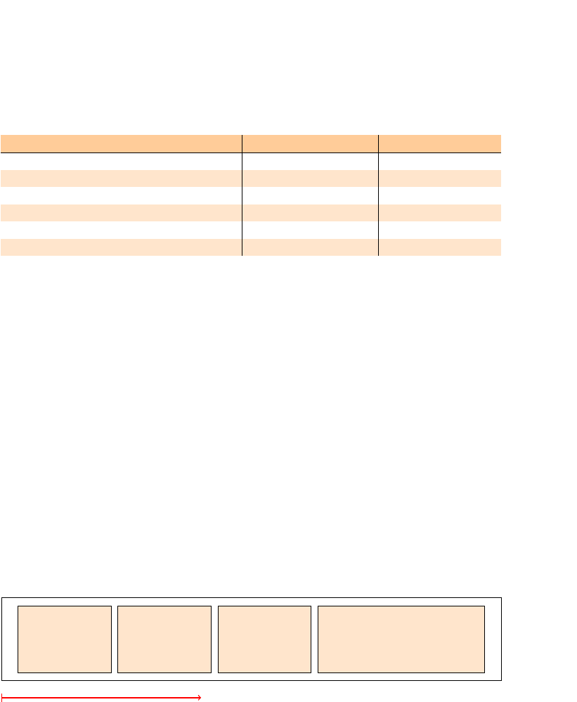
239
There are other special-purpose values for FAT entries, as listed in Figure 9.15. All entries have the
same xed length, as specied by the FAT variant. FAT12 has 12-bit entries, FAT16 has 16-bit, FAT32
has 32-bit.
Figure 9.15: FAT entry values and their interpretaon.
In FAT systems, a directory is a special type of le that consists of mulple entries. Each directory
entry occupies 32 bytes and encodes the name and other metadata of a le (although not as rich as
an inode, generally) along with the FAT index of the rst block of le data.
In earlier FAT formats (i.e., 12 and 16) the root directory occupies the special root directory region.
It is stacally sized when the le system is created, so there is a limited number of entries in the
root directory. For FAT32, the root directory is a general le in the data region so it can be resized
dynamically.
Figure 9.16 shows how the various regions of the FAT le system are laid out on a device. The inial
reserved block is for boot code. The FAT is a xed size, depending on the number of blocks available
in the data region. Each FAT entry is n bytes long, for the FAT-n variant of the le system, where n may
be 12, 16 or 32. For FAT12 and FAT16, as shown in the diagram, the root directory is a disnct, xed-
size region. This is followed by the data region, which contains all other directories and les.
Figure 9.16: Schemac diagram showing regions for a FAT format disk image.
9.12.1 Advantages of FAT
Due to the linked list nature of les, they must be accessed sequenally by chasing pointers from the
start of the le. Since the pointers are all close together (in the FAT, rather than inline in the data blocks)
they have high spaal locality. The FAT is oen cached in RAM, so it is ecient to access and traverse.
FAT is a simple le system in terms of implementaon complexity. Its simplicity, along with its
longevity, explain its widespread deployment.
i
i
“chapter” — 2019/8/13 — 20:50 — page 15 — #15
i
i
i
i
i
i
entry meaning FAT16 value
0 free block 0x0000
1 temporarily non-free 0x0001
2
! (MAXWORD - 16) next block pointer
MAXWORD - 15 ! MAXWORD - 9 reserved values 0xFFF6
MAXWORD - 8
bad block 0xFFF7
MAXWORD - 7
!
MAXWORD end of file marker 0xFFF8
!
0xFFFF
i
i
“chapter” — 2019/8/13 — 20:50 — page 16 — #16
i
i
i
i
i
i
reserved
(boot sector)
file allocation
table
root
directory
data
blocks
logical disk addresses
Chapter 9 | Persistent storage

Operang Systems Foundaons with Linux on the Raspberry Pi
240
9.12.2 Construct a Mini File System using FAT
The best way to understand how a le system works is to construct one for yourself. In this praccal
secon, we will programmacally build a disk image for a simple FAT16 le system, then mount the
image le on a Raspberry Pi system and interact with it.
The Python program shown below will create a blank le system image. Read through this source code
to understand the metadata details required for specifying a FAT le system.
Lisng 9.12.2: Programmacally create a FAT disk image Python
1 # create a binary le
2 f = open('fatexample.img', 'wb')
3
4 ### BOOT SECTOR, 512B
5 # rst 3 bytes of boot sector are 'magic value'
6 f.write( bytearray([0xeb, 0x3c, 0x90]) )
7
8 # next 8 bytes are manufacturer name, in ASCII
9 f.write( 'TEXTBOOK'.encode('ascii') )
10
11 # next 2 bytes are bytes per block - 512 is standard
12 # this is in little endian format - so 0x200 is 0x00, 0x02
13 f.write( bytearray([0x00, 0x02]) )
14
15 # next byte, number of blocks per allocation unit - say 1
16 # An allocation unit == A cluster in FAT terminology
17 f.write( bytearray([0x01]) )
18
19 # next two bytes, number of reserved blocks -
20 # say 1 for boot sector only
21 f.write( bytearray([0x01, 0x00]) )
22
23 # next byte, number of File Allocation tables - can have multiple
24 # tables for redundancy - we'll stick with 1 for now
25 f.write( bytearray([0x01]) )
26
27 # next two bytes, number of root directory entries - including blanks
28 # let's say 16 les for now, so root dir is contained in single block
29 f.write( bytearray([0x10, 0x00]) )
30
31 # next two bytes, number of blocks in the entire disk - we want a 4 MB disk,
32 # so need 8192 0.5K blocks == 2^13 == 0x00 0x20
33 f.write( bytearray([0x00, 0x20]) )
34
35 # single byte media descriptor - magic value 0xf8
36 f.write( bytearray([0xf8]) )
37
38 # next two bytes, number of blocks for FAT
39 # FAT16 needs two bytes per block, we have 8192 blocks on disk
40 # 512 bytes per block - i.e. can store FAT metadata for 256 blocks in
41 # a single block, so need 8192/256 blocks == 2^13/2^8 == 2^5 == 32
42 f.write( bytearray([0x20, 0x00]) )

241
Lisng 9.12.3: Connuaon of FAT disk image creaon Python
1 # next 8 bytes are legacy values, can all be 0
2 f.write( bytearray([0,0,0,0,0,0,0,0]) )
3
4 # next 4 bytes are total number of blocks in entire disk -
5 # ONLY if it overows earlier 2 byte entry otherwise 0s
6 f.write( bytearray([0x00, 0x00, 0x00, 0x00]) )
7
8 # next 2 bytes are legacy values
9 f.write( bytearray([0x80,0]) )
10
11 # magic value 29 - for FAT16 extended signature
12 f.write( bytearray([0x29]) )
13
14 # next 4 bytes are volume serial number (unique id)
15 f.write( bytearray([0x41,0x42,0x43,0x44]) )
16
17 # next 11 bytes are volume label (name) - pad with trailing spaces
18 f.write( "TEST_DISK ".encode('ascii'))
19
20 # next 8 bytes are le system identier - pad with trailing spaces
21 f.write( "FAT16 ".encode('ascii'))
22
23
24 # pad with '\0'
25 for i in range(0,0x1c0):
26 f.write( bytearray([0]) )
27
28 # end of boot sector magic marker
29 f.write( bytearray([0x55, 0xaa]) )
30
31
32 ## FILE ALLOCATION TABLE
33 # each entry needs 2 bytes for FAT16
34 # We need 8192 entries (== 32 blocks of 512B)
35
36 # (a) rst two entries are magic values 0xf8 0x
37 f.write( bytearray([0xf8,0x,0x,0x]))
38
39 # (b) subsequent 8190 FAT entries should be 0x00
40 f.write( bytearray([0x00,0x00]*8190) )
41
42 ## ROOT DIRECTORY AREA
43 # There are 16 les in the root directory
44 # Each le entry occupies 32 bytes - we just no entries for now - all zeros.
45 # Root directory takes 16*32 bytes == 512B == 1 block
46 f.write( bytearray([0x00]*512) )
47
48 ## DATA REGION
49 # create 8192 blank blocks, each containing 512 bytes of zero values
50 for i in range(8192):
51 f.write( bytearray([0x00]*512) )
52
53 ## All done - nally close le
54 f.close()
Chapter 9 | Persistent storage
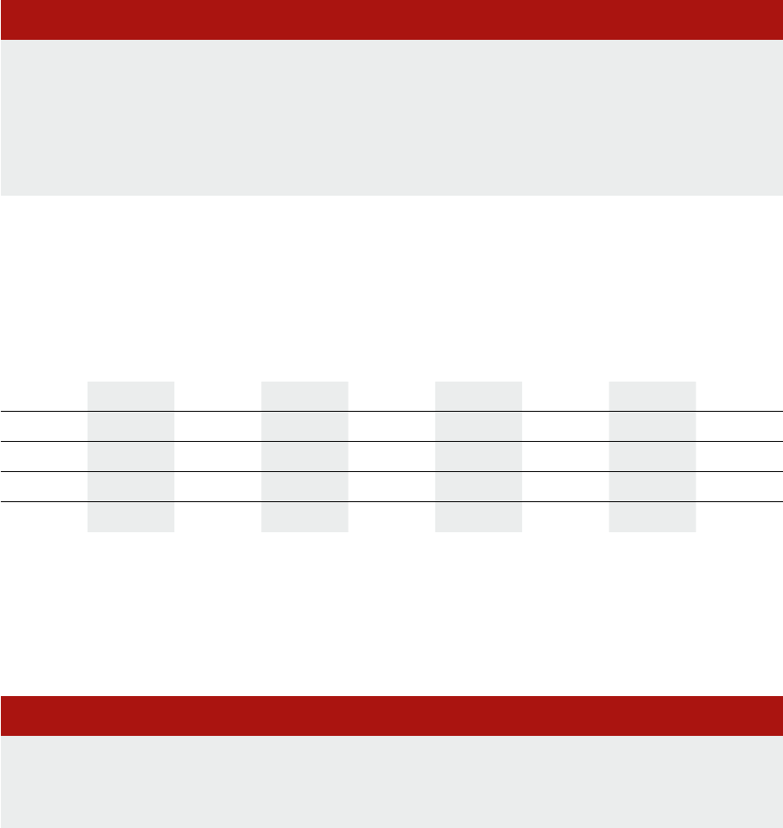
Operang Systems Foundaons with Linux on the Raspberry Pi
242
Lisng 9.12.4: Interacng with the FAT disk image Bash
1 # Step 1: mount the le system
2 sudo mount -t vfat -o loop fatexample.img /mnt
3 # Step 2: add a multiple block le
4 sudo dd if=/usr/share/dict/words of=/mnt/words.txt count=5 bs=512
5 # Step 3: unmount the le system
6 umount /mnt
7 # Step 4: hexdump the le to nd the new le's cluster addresses
8 hexdump -x fatexample.img |less
Inspect the FAT data, which starts at address 0x200 in the le; aer the inial magic vales, subsequent
entries are sequenal cluster numbers, nishing with an end-of-cluster marker.
Because the FAT le system we created is inially blank, the newly allocated le is stored in
consecuve clusters on the disk. Over me, as a FAT le system becomes more used and fragmented,
les may not be consecuve.
When free data blocks are required, the system scans through the FAT to nd the index numbers of
blocks that are marked as free and uses these for fresh le data.
If the Python code above is too long to aempt, you could also use the mkfs tool to create a blank
FAT16 disk image, as shown below.
Lisng 9.12.5: Automacally create a FAT image Bash
1 sudo apt-get install dosfstools # for manipulating FAT images
2 dd if=/dev/zero of=./fat.img bs=512 count=8192 # blank image
3 mkfs.fat -f 1 -F 16 -i 41424344 -M 0xF8 -n TEST_DISK \
4 -r 32 -R 1 -s 1 -S 512 ./fat.img
9.13 Latency reducon techniques
To minimize the overhead of accessing persistent storage, which can have relavely high latency, Linux
maintains an in-memory cache of blocks recently read from or wrien to secondary storage. This is
known as the buer cache. It is sized to occupy free RAM, so it grows and shrinks as other processes
require more or less memory. The contents of the buer cache are ushed to disk at regular intervals,
to ensure consistency.
*
00001f0 0000 0000 0000 0000 0000 0000 0000 aa55
0000200 fff8 ffff 0000 0004 0005 0006 0007 ffff
0000210 0000 0000 0000 0000 0000 0000 0000 0000
*

243
Another technique to reduce latency is the use of a RAM disk. This involves dedicang a poron of
memory to be handled explicitly as part of the le system. It makes sense for transient les (e.g., those
resident in /tmp) or log les that will be accessed frequently. The kernel has specic support for this
mapping of memory to le system, called tmpfs. Create a RAM disk of 50MB size as follows:
Lisng 9.13.1: Create a RAM disk Bash
1 sudo mkdir /mnt/ramdisk
2 sudo mount -t tmpfs -o size=50M newdisk /mnt/ramdisk
Note les in the directory /mnt/ramdisk are not persistent. This directory is lost when the system is
powered down. RAM disks are parcularly useful for embedded devices like the Raspberry Pi, for
which repeated high frequency writes to disk can cause SD card corrupon.
9.14 Fixing up broken le systems
Persistent storage media may be unreliable. Bad blocks should be detected and avoided. File systems
have mechanisms for recording bad blocks to ensure data is not allocated to these blocks. For
instance, FAT has a bad block marker.
Somemes, le systems are in an inconsistent state if the system is powered down unexpectedly, or
devices are removed without unmounng. Some data may have been cached in RAM, but not wrien
back to disk before the shutdown or removal.
Fixup ulies like fsck can check and repair le system glitches. They check for directory integrity and
make alteraons (e.g., to inode reference counts) as appropriate. File System journals may be used to
replay incomplete acons on le systems.
These general-purpose tools can handle many common le system problems. For more serious issues,
expert cyber forensic tools are available. These facilitate paral data recovery from damaged devices.
9.15 Advanced topics
Some storage media are read-only, such as opcal disks. On Linux, any le system may be mounted
for read-only access. This implies that only certain operaons are permied, and no metadata updates
(even access mestamps) are possible. Generally, read-only media have specialized le system formats
such as the universal disk format (UDF) for DVDs.
Specialized Raspberry Pi Linux distribuons may mount the root le system as read-only, with any le
writes directed to transient RAM disk storage. This is an aempt to guarantee system integrity, e.g.,
for public display terminals in museums.
Network le systems are commonplace, parcularly given widespread internet connecvity.
In addion to the issues outlined above for local le systems, network le system protocols must
also handle:
Chapter 9 | Persistent storage

Operang Systems Foundaons with Linux on the Raspberry Pi
244
1. Distributed access control: global user idenes are managed and authencated in the system.
2. High and variable latency: underlying data may be stored in remote locaons over a wide area
network, with clients experiencing occasional lack of connecvity.
3. Consistency: mulple users may concurrently access and modify a shared, possibly replicated,
resource.
A union le system, also known as an overlay le system, is a transparent composion of two disnct
le systems. The base layer, oen a read-only system like a live boot CD, is composed with an upper
layer, oen a writeable USB sck. Overlays are also extensively used for containerizaon, in systems
like Docker. From user space, the union appears to be a single le system. The lisng below shows
how you can set up a sample union le system on your Raspberry Pi. If you inspect the lower layer, it
is not aected by modicaons in the merged layer. The upper layer acts like a ‘le system di’ applied
to the lower layer.
Lisng 9.15.1: A sample union le system Bash
1 cd /tmp
2 # set up directories
3 mkdir lower
4 echo "hello" > a.txt
5 touch b.txt
6 mkdir upper
7 mkdir work
8 mkdir merged
9 sudo mount -t overlay overlay -olowerdir=/tmp/lower,\
10 upperdir=/tmp/upper,workdir=/tmp/work /tmp/merged
11 cd merged
12 echo "hello again" >> b.txt
13 touch c.txt
14 ls
15 ls ../upper
16 ls ../lower
Standard, concrete le system implementaons are built into the kernel, or loaded as kernel modules.
The goal of the FUSE project is to enable le systems in user space. FUSE consists of:
1. A small kernel module that mediates with VFS on behalf of non-privileged code.
2. An API that can be accessed from user space.
FUSE enables more exibility for development and deployment of experimental le systems. Mulple
high-level language bindings available, allowing developers to create le systems in languages as
diverse as Python and Haskell.

245
9.16 Further reading
The ext4 le system is introduced, movated, and empirically evaluated in a paper [1] by some of its
development team. There are a number of helpful illustraons in this paper. It also includes details on
high-level design decisions that underpin ext4.
The wiki page at hp://ext4.wiki.kernel.org features a comprehensive collecon of online resources
about ext4.
The detailed coverage of VFS and legacy ext2/ext3 le systems in the O’Reilly textbook on
Understanding the Linux Kernel [2] is well worth reading. The authors provide much more detail,
including relevant commentary on kernel source code data structures and algorithms.
9.17 Exercises and quesons
9.17.1 Hybrid Conguous and linked le system
Consider a block-structured le system where the rst N blocks of a le are arranged conguously,
and then subsequent blocks are linked together in a linked list data structure (like FAT). What are the
advantages of this le system organizaon? What are the potenal disadvantages?
9.17.2 Extra FAT le pointers
Consider a linked le system, like FAT. The directory entry for each le has a single pointer to the rst
block of the le. Why might it be a good idea to keep a second pointer, to the nal block of the le?
Which operaons would have their eciency improved?
Imagine a FAT style system with doubly linked lists, i.e., each FAT entry has pointers to both the next
and previous blocks. Would this improve le seek mes, in general? Do you think the space overhead
is acceptable?
9.17.3 Expected le size
Inspect your ext4 root le system. See how much space is available on it with df -h. Then see how
many inodes are free with df -i. Use these results to calculate the expected space to be occupied by
each future le, assuming a single inode per le (i.e., no mulple links).
9.17.4 Ext4 extents
This queson concerns the relave merits of ext4 style extents in comparison to tradional block
map indexing. Consider creang and wring data to an N-block le, where the data blocks are laid out
conguously on disk. How many bytes would need to be wrien for extent-based locaon metadata?
How many bytes would need to be wrien for a block map index? When might a block map index be
more ecient than extent-based metadata?
9.17.5 Access mes
Create a RAM disk, using the commands outlined above. Now plug in a USB drive. Compare the write
latencies for both devices, by wring a 100MB le of random data to them. Use the dd command with
source data from /dev/urandom. Which device has lower latency, and why? You might also compare
these mes with wring 100MB to your Pi SD card.
Chapter 9 | Persistent storage
Operang Systems Foundaons with Linux on the Raspberry Pi
246
9.17.6 Database decisions
Imagine you have to architect a big data storage system to run on the Linux plaorm. You can choose
between:
1. A massive single monolithic data dump le
2. A set of small les, each of which stores a single data record
Discuss the implementaon trade-os involved in this decision. Which alternave would you select,
and why?
References
[1] A. Mathur, M. Cao, S. Bhaacharya, A. Dilger, A. Tomas, and L. Vivier, “The new ext4 le system: current status and future
plans,” in Proceedings of the Linux Symposium, vol. 2, 2007, pp. 21–33.
[2] D. P. Bovet and M. Cesa, Understanding the Linux Kernel, 3rd ed. O’Reilly, 2005.

247
Chapter 9 | Persistent storage

Chapter 10
Networking

Operang Systems Foundaons with Linux on the Raspberry Pi
250
10.1 Overview
This chapter will introduce networking from an operang systems perspecve. We discuss why
networking is treated dierently from other types of I/O and what the operang system requirements
are to support networking. We introduce POSIX socket programming both in terms of the role the
OS plays (e.g., socket buers, le abstracon, supporng mulple clients,.) as well as from a praccal
perspecve.
The focus of this book is not on networking per se; we refer the reader to the standard textbooks by
Peterson and Davies [1] or Tanenbaum [2] or the open source book [3] by Bonaventure
1
.
What you will learn
Aer you have studied the material in this chapter, you will be able to:
1. Explain the role of the Linux kernel in networking.
2. Discuss the relaonship between and structure of the Linux networking stack and the kernel
networking architecture.
3. Use the POSIX API for programming networking applicaons: data types, common API and ulity
funcons.
4. Build TCP and UDP client/server applicaons and handle mulple clients.
10.2 What is networking
When we say "networking," we refer to the interacon of a computer system with other computer
systems using an intermediate communicaon infrastructure. In parcular, our focus will be on the
TCP/IP protocol and protocols implemented on top of TCP/IP such as HTTP; and to a lesser extent
on the wired (802.3) and wireless (802.11) Ethernet media access control (MAC) protocols.
10.3 Why is networking part of the kernel?
The network interface controller (NIC, aka network adapter) is a peripheral I/O device . Therefore,
as with all peripherals, access to this device is controlled via a device driver which must be part of
the kernel. However, why does the kernel also implement the TCP/IP protocol suite? Why does it
not leave this to user space and simply deliver the data as received by the NIC straight to the user
applicaon?
And indeed, there are a number of user space TCP/IP implementaons [4, 5, 6, 7]. Some of these
claim to outperform the Linux kernel TCP/IP implementaon, but the performance of the Linux kernel
network stack has improved considerably, and version 4.16 (the current kernel at the me of wring)
contained a lot of networking changes.
1
Available at hp://cnp3book.info.ucl.ac.be/
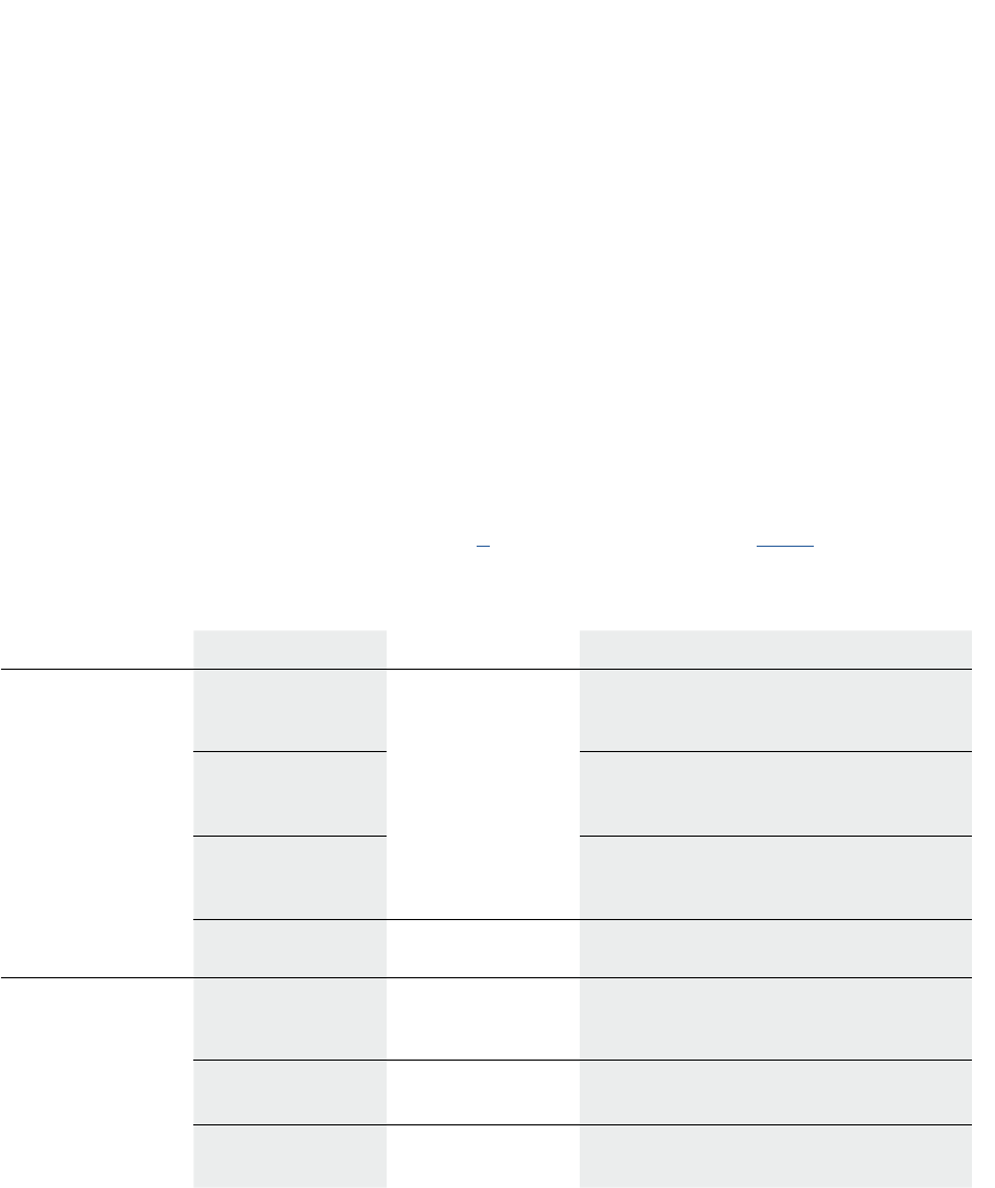
251
However, there are two main reasons to put networking in the kernel:
If we would not do this, only a single process at a me could have access to the network card. By
using the kernel network stack, we have the ability to run mulple network applicaons, servers
as well as clients. Achieve the same result eciently in user space is impossible because a process
cannot preempt another process like the OS scheduler can.
Furthermore, there is the issue of control over the incoming packets. Unlike other peripherals,
which are typically an integral part of the system and enrely under control of the user, the NIC
delivers data from unknown sources. If we would delegate the networking funconality to user
space, then the kernel couldn’t act as the controller of the incoming (and outgoing) data.
10.4 The OSI layer model
Communicaon networks have tradionally been represented as layered models. In parcular, the OSI
(Open Systems Interconnecon) reference model [8], ocially the ITU standard X.200, is very widely
known. A shown in Table 10.1), this model consists of seven layers. The protocol data unit (PDU) is
informaon that is transmied as a single unit among peer enes of a computer network.
Table 10.1: OSI layer model.
The upper four layers, Applicaon, Presentaon, Session, and Transport, are known as the “Host
layers.” They are responsible for accurate and reliable data delivery between applicaons in computer
systems. They are called “host” layers because their funconality is implemented—at least in
principle—solely by the host systems, and the intermediate systems in the network don’t need to
Layer Protocol data unit Funcon
Host layers 7. Applicaon Data The sole means for the applicaon process to access
the OSI environment, i.e., all OSI services directly
usable by the applicaon process.
6. Presentaon Representaon of informaon communicated
between computer systems. This could, for example,
include encoding, compression, and encrypon.
5. Session Control of the connecons between computer
systems. Responsible for session management,
including checkpoinng and recovery.
4. Transport Segment, Datagram Transparent transfer of data, including reliability,
ow control, and error control.
Media layers 3. Network Packet Funconality to transfer packets between computer
systems. In pracce, this means the roung protocol
and the packet format.
2. Data link Frame Funconality to manage data link (i.e. node-to-node)
connecons between computer systems.
1. Physical Symbol Actual hardware enabling the communicaon
between computer systems as raw bitstreams.
Chapter 10 | Networking
Operang Systems Foundaons with Linux on the Raspberry Pi
252
implement these layers. The lower three layers, Network, Data Link and Physical, are known as “Media
layers” (short for communicaons media layer). The media layers are responsible for delivering the
informaon to the desnaon for which it was intended. The funconality of these layers is typically
implemented in the network adapter.
10.5 The Linux networking stack
In pracce, the Session and Presentaon layers are not present as disnct layers in the typical TCP/IP
based networking stack. A praccal layer model for the TCP/IP protocol suite is shown in Figure 10.1.
Figure 10.1: Layer model for the TCP/IP protocol suite.
The Linux kernel provides the link layer, network layer, and transport layer. The link layer is
implemented through POSIX-compliant device drivers; the network and transport layers (TCP/IP)
are implemented in the kernel code. In the next secons, we provide an overview of the Linux kernel
networking architecture (Figure 10.2).
Figure 10.2: Linux kernel networking architecture.
Hardware layer
Link layer
Network layer
Transport layer
Application layer
User/Application
Ethernet
Ethernet driver
IP, IPv6 protocols
TCP, UDP protocol
HTTP, SMTP, SSL protocols
Web browser, email client
ExampleNetwork stack
User space
Kernel space
Network Interface Controller (NIC)
Device-agnostic interface
Network protocols (INET)
Application layer
User space
Kernel space
System call interface
Hardware
Device drivers
Protocol-agnostic interface

253
10.5.1 Device drivers
The physical network devices (NIC) are managed by device drivers. For what follows, we assume the
NIC is an Ethernet device. The device driver is a soware interface between the kernel and the device
hardware. On the kernel side, it uses a low-level but standardized API so that any driver for a dierent
NIC can be used in the same way. In other words, the device driver abstracts away as much as possible
the specic hardware.
The normal le operaons (read, write, ...) do not make sense when applied to the interacon between
a driver and a NIC, so they do not follow the "everything is a le" philosophy. The main dierence is
that a le, and by extension a le storage device is passive, whereas a network device acvely wants
to push incoming packets toward the kernel. So NIC interrupts are not a result of a previous kernel
acon (as is the case with, e.g. le operaons), but of the arrival of a packet. Consequently, network
interfaces exist in their own namespace with a dierent API.
10.5.2 Device-agnosc interface
The network protocol implementaon code interfaces with the driver code through an agnosc
interface layer which allows us to connects various protocols to a variety of hardware device drivers.
To achieve this, the calls work on a packet-by-packet basis so that it is not necessary to inspect the
packet content or keep protocol-specic state informaon at this level. The interface API is dened in
linux/net/core/dev.c. The actual interface is a struct of funcon pointers called net_- device_ops,
dened in include/linux/netdevice.h. In the driver code, the applicable elds are populated using
driver-specic funcons.
10.5.3 Network protocols
Packets get handed over the actual network protocol funconality in the kernel. For our purpose, we
focus on the TCP/IP protocol, known in the Linux kernel as inet. This is a whole suite of protocols, the
best-known of which are IP, TCP, and UDP. The code for this can be found in net/ipv4 for IP v4 and in
net/ipv6 for IP v6.
In parcular, IPv4 protocols are inialized in a inet_init() (dened in linux/net/ipv4/af_inet.c). This
funcon registers each of the built-in protocols using the proto_register() funcon (dened in linux/net/
core/sock.c). It adds the protocol to the acve protocol list and also oponally allocates one or more
slab caches. The Linux kernel implements a caching memory allocator to hold caches (called slabs)
of idencal objects. A slab is a set of one or more conguous pages of memory set aside by the slab
allocator for an individual cache.
10.5.4 Protocol-agnosc interface
The network protocols interface with a protocol-agnosc layer that provides a set of common
funcons to support a variety of dierent protocols. This layer is called the sockets layer, and it
supports not only the common TCP and UDP transport protocols but also the IP roung protocol,
various Ethernet protocols, and others, e.g., Stream Control Transmission Protocol (SCTP). We will
discuss the POSIX socket interface in more detail in secon 10.6.
The socket interface is an abstracon for the network connecon. The socket datastructure contains
all of the required state of a parcular socket, including the parcular protocol used by the socket
and the operaons that may be performed on it. The networking subsystem knows about the
Chapter 10 | Networking
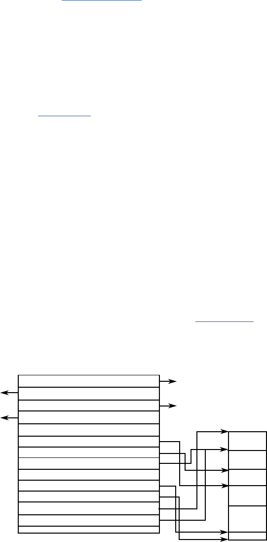
Operang Systems Foundaons with Linux on the Raspberry Pi
254
available protocols through a special structure that denes its capabilies. Each protocol maintains a
(large) structure called proto (dened in include/net/sock.h). This struct denes the parcular socket
operaons that can be performed from the sockets layer to the transport layer (for example, how to
create a socket, how to establish a connecon with a socket, how to close a socket, etc.).
10.5.5 System call interface
We have covered the Linux system call interface in Chapter 5. Essenally, this is the interface
between user space and kernel space. Recall that Linux system calls are idened by a unique
number and take a variable number of arguments. When a networking call is made by the user,
the system call interface of the kernel maps it to a call to sys_socketcall (dened as SYSCALL_-
DEFINE2(socketcall,...) in net/socket.c), which then further demulplexes the call to its
intended target, e.g., SYS_SOCKET, SYS_BIND, etc.
It is also possible to use the le abstracon for networking I/O. For example, typical read and write
operaons may be performed on a networking socket (which is represented by a le descriptor, just
as a normal le). Therefore, while there exist a number of operaons that are specic to networking
(creang a socket with the socket call, connecng it to a desnaon with the connect call, and so on),
there are also a number of standard le operaons that apply to networking objects just as they do
to regular les.
10.5.6 Socket buers
A consequence of having many layers of network protocols, each one using the services of another,
is that each protocol needs to add protocol headers (and/or footers) to the data as it is transmied and
to remove them as packets are received. This could make passing data buers between the protocol
layers dicult as each layer would need to nd where its parcular protocol headers and footers are
located within the buer. Copying buers between layers would, of course, work, but it would be very
inecient. Instead, the Linux kernel uses socket buers (a.k.a. sk_bus) (struct sk_bu) to pass data
between the protocol layers and the network device drivers. Socket buers contain pointer and length
elds that allow each protocol layer to manipulate the applicaon data via standard funcons.
Figure 10.3: Socket buer structure.
struct sk_buff *next
struct sk_buff *prev
struct sock *sk
struct net_device *dev
...
__u16 mac_header
__u16 network_header
__u16 transport_header
*sk_buff
*sk_buff
struct sk_buff
sock
structure
device (NIC)
sk_buff_data_t tail
sk_buff_data_t end
unsigned char *head
unsigned char *data
...
MAC
IP
TCP
Packet

255
Essenally, an sk_bu combines a control structure with a block of memory. Two main sets of
funcons are provided in the sk_bu library: the rst set consists of rounes to manipulate doubly
linked lists of sk_bus; the second set of funcons for controlling the aached memory. The buers
are stored in linked lists opmized for the common network operaons of append to end and remove
from start. In pracce, the structure is quite complicated (the complete struct comprises 66 elds).
Figure 10.3 shows a simplied diagram of the sk_bu struct.
10.6 The POSIX standard socket interface library
In this secon, we present some of the most useful POSIX standard socket interface library funcons
and the related internet data types and constants. The selecon focuses on IPv4 TCP stream sockets.
10.6.1 Stream socket (TCP) communicaons ow
The Transmission Control Protocol is a core protocol in the TCP/IP stack and implements one of
the two transport layer (OSI layer 4) protocols (the other being UDP, the User Datagram Protocol).
All incoming IP network layer packets marked with the relevant TCP idener in the IP protocol ID header
eld are passed upwards to TCP, and all outgoing TCP packets are passed down to the IP layer for sending.
In turn, TCP is responsible for idenfying the (16-bit) port number from the TCP packet header and
forwarding the TCP packet payload to any acve socket associated with the specied port number.
TCP is reliable and connecon-oriented and as such employs various handshaking acvies in the
background between the TCP layers in the communicang nodes to handle the setup, reliability
control and shutdown of the TCP connecon. The socket API provides a simplied programming
model for the TCP to applicaon interface, and the connected stream sockets can be considered
as the communicaon endpoints of a virtual data circuit between two processes.
To establish a socket connecon, one of the communicang processes (the server) needs to be acvely
waing for a connecon on an acve socket and the other process (the client) can then request
a connecon and if successful the connecon is made. The meline of the various socket library
funcon calls required in a typical (simple) stream socket connecon is shown below:
Server meline Client meline Descripon
1. Socket(. . . ) Server creates a socket le descriptor
2. Setsockopt(. . . ) Congure server socket protocol opons (1 call per opon)
3. Bind(. . . ) Associate the server socket with a predened local port number
4. Listen(. . . ) Allow client connecons on the server socket
5. Accept(. . . ) Wait for client connecon request
1. Socket(. . . ) Client creates a socket le descriptor
2. Connect(. . . ) Client requests connecon to the server socket
6. Recv(. . . )/send(. . . ) 3. Recv(. . . )/send(. . . ) Client/Server data communicaons
7. Close(. . . ) 4. Close(. . . ) Either process can close the stream socket connecon rst
Chapter 10 | Networking

Operang Systems Foundaons with Linux on the Raspberry Pi
256
Treang stream sockets as standard system devices: read()/write()
The read() and write() low level I/O library funcons are not part of the standard socket
library; however stream sockets behave in much the same manner as any other operang
system device (standard input/output, le, etc) and low-level system device I/O operaons
are therefore compable with stream socket I/O. The use of these funcons in place of the
standard socket library funcons send(), and recv() (used for stream sockets only) is a common
programming nicety that will allow the simple redirecon of process communicaons from
network to any other available I/O device in the host OS. In comparison; the standard socket
library funcons sendto() and recvfrom() used for datagram sockets (UDP) are not compable
with the low-level stream I/O due to their unreliable and conneconless characteriscs and
therefore cannot be treated in the same way.
Note
A read from a stream socket (using the read() or recv() funcons) may not return all of the
expected bytes in the rst go, and the read operaon may need to be repeated an unspecied
number of mes with the read results concatenated unl the full number of expected bytes has
been received. If the expected number of bytes is not known in advance, the stream should be
read a small block of bytes (possible 1 byte) at a me unl the receive count is idened using
a data size eld within the received data or a predened data terminator sequence. It is up to
the individual internet applicaon to dene any data size eld syntax and/or data terminators
used. Aempng to read more data that has been sent will block the read() or recv() funcon
call which will hang waing for new data.
10.6.2 Common Internet data types
As menoned previously — only the stream socket related library funcons and associated data types
and constants are listed here. Due to target dierences in the fundamental integer data types ulised
between various implementaons of the standard socket interface — the POSIX dened types ‘u_char’
(8-bit), ‘u_short’ (16-bit) and ‘u_long’ (32-bit) (normally declared in ‘sys/types.h’ for UNIX systems)
are used here to signify xed word length integer data types and may be ulized in any required
programming type casts.
The following secons discuss some reference material for useful standard socket interface library
funcons and internet data types.
Socket address data type: struct sockaddr
The socket address data structure used in various socket library funcon calls is dened in sys/socket.h as:
Lisng 10.6.1: socket address struct C
1 struct sockaddr {
2 u_char sa_family; /* address family */
3 char sa_data[14]; /* value of address */
4 };

257
Internet socket address data type: struct sockaddr_in
The members of the socket address data structure do not seem to relate much to what we would
expect for an internet address (and port number). This is due to the fact that the socket interface is
not restricted to internet communicaons and many alternave underlying host to host transport
mechanisms are available (specied by the value of the ‘sa_family’ socket address structure member),
and these have dierent address schemes that have to be supported. The 14-byte address data is
formaed in dierent ways depending on the underlying transport. For simplicity; a specic internet
socket address structure has also been dened which is used as an overlay to the more generic socket
address structure. This makes programming the address informaon much more convenient as
a template for the specic internet address value format is provided:
Lisng 10.6.2: internet socket address struct C
1 #include <netinet/in.h>
2 struct sockaddr_in {
3 sa_family_t sin_family; /* address family: AF_INET */
4 in_port_t sin_port; /* port in network byte order */
5 struct in_addr sin_addr; /* internet address */
6 };
The internet socket address structure has the member type struct in_addr:
Lisng 10.6.3: internet address struct (IPv4) C
1 #include <netinet/in.h>
2
3 struct in_addr {
4 uint32_t s_addr; /* address in network byte order */
5 };
When using a variable of internet socket address type, it is good pracce to zero-ll the overlay
padding sin_zero.
Network byte order versus host byte order
The network byte order for TCP/IP is dened as big-endian; this is reected in the data types
used in the standard socket interface library. As such it is essenal that the host byte order
is correctly mapped to the network byte order when seng values of the standard socket
data type variables used and vice versa when interpreng these values. The htons() and htonl()
funcons are used to convert host byte order 16-bit and 32-bit data types to their respecve
network byte order and ntohs() and ntohl() funcons are used to convert network byte order
16-bit and 32-bit data types to their respecve host byte order. This feature of standard
socket programming is a minor but essenal aspect to ensure the portability of internet
applicaon code.
Arm plaorms can be congured to run in lile-endian or big-endian mode at boot me, so it is
essenal to use the above conversion funcons to ensure correctness of the code.
Chapter 10 | Networking

Operang Systems Foundaons with Linux on the Raspberry Pi
258
10.6.3 Common POSIX socket API funcons
Create a socket descriptor: socket()
A socket (socket(2)) is opened, and its descriptor created using:
Lisng 10.6.4: socket() API call C
1 #include <sys/types.h> /* See NOTES */
2 #include <sys/socket.h>
3
4 int socket(int domain, int type, int protocol);
Return value: the returned socket descriptor is a standard I/O system le descriptor and can also be
used with the I/O funcons: close() and in the case of stream type sockets with read()’ and ‘write().’
On error, the value -1 is returned.
Input parameters: The address family parameter domain should be set to AF_INET for internet
socket communicaons. The socket type parameter type should be selected from SOCK_STREAM
or SOCK _DGRAM for stream (TCP) and datagram (UDP) sockets respecvely. The protocol family
parameter family can be set to 0 to allow the socket funcon to select the associated protocol family
automacally.
Bind a server socket address to a socket descriptor: bind()
For ‘server’ type applicaons (i.e., those that listen for incoming connecons on an opened socket) the
server socket address is bound to a socket descriptor using bind(2):
Lisng 10.6.5: bind() API call C
1 #include <sys/types.h> /* See NOTES */
2 #include <sys/socket.h>
3 int bind(int sockfd, const struct sockaddr *addr,
4 socklen_t addrlen);
Return value: the funcon returns 0 on success or -1 if the socket is invalid, the specied socket
address is invalid or in use or the specied socket descriptor is already bound.
Input parameters: typically for internet server type applicaons an internet socket address is used for
convenience when specifying the local socket address; however since the internet socket address
structure is designed as an overly to the generic socket address structure — variables of type struct
sockaddr_in can be passed as the addr parameter using a suitable type cast. Before calling the bind()
funcon it is necessary to populate the internet socket address (shown as myaddr below) with the
local system IP address and the required server port number:

259
Lisng 10.6.6: populang the internet socket address for bind() C
1 mysd = socket(AF_INET, SOCK_STREAM, 0);
2 memset((char *) &myaddr, 0, sizeof(struct sockaddr_in)); /* zero socket address */
3 myaddr.sin_len = (u_char) sizeof(struct sockaddr_in); /* address length */
4 myaddr.sin_family = AF_INET; /* internet family */
5 myaddr.sin_addr.s_addr = inet_addr("192.168.0.10"); /* local IP address */
6 myaddr.sin_port = htons(3490); /* local server port */
7 bind(mysd, (struct sockaddr_in *) &myaddr, sizeof(struct sockaddr) );
Note the use of ‘memset()’ from the ANSI string library to rst zero the internet socket address bytes
and the internet address manipulaon funcon inet_addr() to produce the (network byte order) 4 byte
IP address. Using the specic port number 0 tells bind() to choose a suitable unused port — if that is
desired rather than having a xed server port allocaon (the selected port gets wrien to the supplied
socket address before return). Wring the specic local IP address is not very convenient, and the
code can ulmately be made more portable using the INADDR_ANY predened IP address (declared
for use with struct sockaddr_in) which tells bind() to use the local system IP address automacally
(which is also wrien to the supplied socket address before return). Therefore, the server local IP
address is more typically set using:
myaddr.sin_addr.s_addr = htonl(INADDR_-
ANY); /* auto local IP address */
Enable server socket connecon requests: listen()
Once a server socket descriptor has been bound to a socket address it is then necessary to enable
connecon requests to this socket and create an incoming connecon request queue using listen(2):
Lisng 10.6.7: listen() API call C
1 #include <sys/types.h> /* See NOTES */
2 #include <sys/socket.h>
3
4 int listen(int sockfd, int backlog);
Return value: the funcon returns 0 if okay or -1 if the socket is invalid or unable to listen.
Input parameters: incoming connecon requests are queued unl accepted by the server. The parameter
backlog is used to specify the maximum length of this queue and should have a value of at least 1.
Accept a server socket connecon request: accept()
Server socket connecon requests are accepted using accept(2):
Lisng 10.6.8: accept() API call C
1 #include <sys/types.h> /* See NOTES */
2 #include <sys/socket.h>
3
4 int accept(int sockfd, struct sockaddr *addr, socklen_t *addrlen);
Chapter 10 | Networking

Operang Systems Foundaons with Linux on the Raspberry Pi
260
Return value: the funcon returns the newly created socket descriptor associated with the client
socket address on success or -1 on error.
Input parameters: a socket address structure variable (more likely of type struct sockaddr_in with
a suitable type cast) is provided as parameter addr and is used to record the socket address associated
with the socket descriptor of the accepted incoming connecon request which is returned on success.
A pointer to an integer containing the socket address structure length is provided as parameter
addrlen, and this integer variable should contain the length of the socket address structure on input
and is modied to the actual address bytes used on return.
On success, the returned client socket descriptor can be used by the server to send and receive data
to the client.
If no pending connecons are present on the queue, and the socket is not marked as nonblocking,
accept() blocks unl a connecon is present. If the socket is marked nonblocking and no pending
connecons are present on the queue, accept() fails with the error EAGAIN or EWOULDBLOCK.
Linux kernel implementaon of accept()
If the accept() is blocking, the kernel will take care of sleeping the caller unl the call returns. The
process will be added to a wait queue and then suspended unl a TCP connecon request is received.
Once a connecon request has been received, the sock data structure is returned to the socket layer.
The le descriptor number of the new socket is returned to the process as the return value of the
accept() call.
Client connecon request: ‘connect()’
For ‘client’ type applicaons (i.e., those that connect to an acve server socket) a connecon request
to a specied server socket address is made using connect(2):
Lisng 10.6.9: connect() API call C
1 #include <sys/types.h> /* See NOTES */
2 #include <sys/socket.h>
3
4 int connect(int sockfd, const struct sockaddr *addr,
5 socklen_t addrlen);
Return value: the funcon returns 0 on success or -1 on error.
Input parameters: typically for internet client type applicaons an internet socket address is used for
convenience when specifying the remote server socket address; however since the internet socket
address structure is designed as an overly to the generic socket address structure — variables of type
struct sockaddr_in can be passed as the addr parameter using a suitable type cast. Before calling the
connect() funcon, it is necessary to populate the internet socket address (shown as srvaddr below)
with the remote server system IP address and the required server port number:

261
Lisng 10.6.10: populang the internet socket address for connect() C
1 srvsd = socket(AF_INET, SOCK_STREAM, 0);
2 memset((char *) &srvaddr,0, sizeof(struct sockaddr_in)); /* zero socket address */
3 srvaddr.sin_len = (u_char) sizeof(struct sockaddr_in); /* address length */
4 srvaddr.sin_family = AF_INET; /* internet family */
5 srvaddr.sin_addr.s_addr = inet_addr("192.168.0.10"); /* server IP address */
6 srvaddr.sin_port = htons(3490); /* server port */
7 connect(srvsd, (struct sockaddr_in *) &srvaddr, sizeof(struct sockaddr) );
On success, the socket descriptor used in the connecon request can be used by the client to send
and receive data to the server.
Write data to a stream socket: send()
Data is wrien to a stream socket using send(2):
Lisng 10.6.11: send() API call C
1 #include <sys/types.h>
2 #include <sys/socket.h>
3
4 ssize_t send(int sockfd, const void *buf, size_t len, intags);
5 ssize_t sendto(int sockfd, const void *buf, size_t len, intags,
6 const struct sockaddr *dest_addr, socklen_t addrlen);
7 ssize_t sendmsg(int sockfd, const struct msghdr *msg, intags);
Return value: the funcon returns the actual number of bytes sent or -1 on error.
Input parameters: in-stream sockets the socket transport protocol bitwise ags of MSG_OOB (send
as urgent) and MSG_DONTROUTE (send without using roung tables) can be used (mulple bitwise
ags can be set concurrently by OR’ing the selecon). For standard data sending the value 0 is used
for parameter ags.
Because of the stream socket operaon compability with system I/O device operaon, the send()
socket-specic funcon is somemes replaced with the generic write() system I/O funcon. This
means that data sending can be easily redirected to other system devices (such as an opened le or
standard output).
Read data from a stream socket: recv()
Data is wrien to a stream socket using recv(2):
Lisng 10.6.12: recv() API call C
1 #include <sys/types.h>
2 #include <sys/socket.h>
3
4 ssize_t recv(int sockfd, void *buf, size_t len, intags);
5 ssize_t recvfrom(int sockfd, void *buf, size_t len, intags,
6 struct sockaddr *src_addr, socklen_t *addrlen);
7 ssize_t recvmsg(int sockfd, struct msghdr *msg, intags);
Chapter 10 | Networking
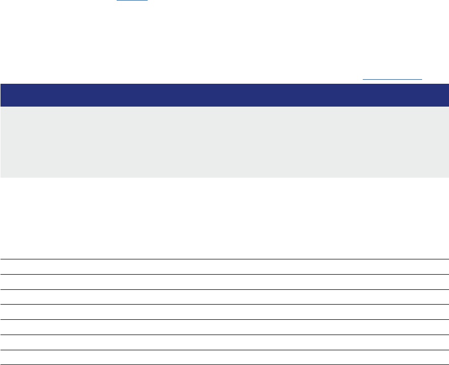
Operang Systems Foundaons with Linux on the Raspberry Pi
262
Return value: the funcon returns the actual number of bytes read into the receive buer; or
0 on end of le (socket disconnecon); or -1 on error.
Input parameters: in-stream sockets the socket transport protocol bitwise ags of MSG_OOB (receive
urgent data) and MSG_PEEK (copy data without removing it from the socket) can be used (mulple
bitwise ags can be set concurrently by OR-ing the selecon). For standard data recepon, the value 0
is used for parameter ags.
Because of the stream socket operaon compability with system I/O device operaon, the recv()
socket specic funcon is somemes replaced with the generic read() system I/O funcon. This
means that data recepon can be easily redirected to other system devices (such as an opened le
or standard input). Care should be taken when reading an expected number of bytes; the socket
transport does not guarantee when to receive bytes will be available, and blocks may be split into
smaller receive secons which may confound a simple socket read approach.
If no messages are available at the socket, the recv() call waits for a message to arrive, unless the
socket is nonblocking (see fcntl(2)), in which case the value -1 is returned and the external variable
errno is set to EAGAIN or EWOULDBLOCK. The recv() call normally returns any data available, up
to the requested amount, rather than waing for receipt of the full amount requested. Therefore in
pracce, recv() is usually called in a loop unl the required number of bytes has been received.
Seng server socket opons: setsockopt()
It is possible to set important underlying protocol opons for a server socket using setsockopt(2):
Lisng 10.6.13: setsockopt() API call C
1 #include <sys/types.h> /* See NOTES */
2 #include <sys/socket.h>
3 int getsockopt(int sockfd, int level, int optname,
4 void *optval, socklen_t *optlen);
5 int setsockopt(int sockfd, int level, int optname,
6 const void *optval, socklen_t optlen);
Return value: the funcon returns 0 on success or -1 if the socket is invalid, or the opon is unknown,
or the funcon is unable to set the opon.
Input parameters:
Socket Opon Used For
SO_KEEPALIVE
Detecng dead connecons (connecon is dropped if dead)
SO_LINGER
Graceful socket closure (does not close unl all pending transacons complete)
TCP_NODELAY
Allowing immediate transmission of small packets (no congeson avoidance)
SO_DEBUG
Invoking debug recording in the underlying protocol soware module
SO_REUSEADDR
Allows socket reuse of port numbers associated with “zombie“ control blocks
SO_SNDBUF
Adjusng the maximum size of the send buer
SO_RCVBUF
Adjusng the maximum size of the receive buer
SO_RCVBUF
Enabling the use of the TCP expedited data transmission.

263
The most commonly applied socket opon for internet server applicaons is the socket reuse address
opon which is required to allow the server to bind a socket to a specic port that has not yet been
enrely freed by a previous session. Without this seng, any call to bind() may be prevented by a
“zombie” session. In order to set this opon, the dened SOL_SOCKET (socket protocol level) is used
for parameter level; the SO_REUSEADDR (the predened name of socket reuse address opon) is
used for parameter optname and for this opon the value is an integer which is set to 0 (OFF) or 1
(ON). A simple example of this for the myfd server socket descriptor is shown below:
Lisng 10.6.14: Example setsockopt() API call C
1 sra_val = 1;
2 setsockopt(myfd, SOL_SOCKET, SO_REUSEADDR, (char *) &sra_val, sizeof(int))
Many other protocol opons are available, see the man page for more details.
10.6.4 Common ulity funcons
Internet address manipulaon funcons
The following internet address manipulaon funcons are available:
Lisng 10.6.15: Internet address manipulaon funcons C
1 #include <arpa/inet.h>
2 /* converts dotted decimal IP address string */
3 /* to network byte order 4 byte value */
4 u_long inet_addr(char * addr);
5 /* converts network byte order 4 byte IP addr*/
6 /* to dotted decimal IP address string */
7 char *inet_ntoa(struct in_addr addr);
Internet network/host byte order manipulaon funcons
The following network/host byte order manipulaon funcons are available and should be
consistently applied:
Lisng 10.6.16: Network/host byte order manipulaon funcons C
1 #include <netinet/in.h>
2 u_short htons(u_short x); /* 16-bit host to network byte order convert */
3 u_short ntohs(u_short x); /* 16-bit network to host byte order convert */
4 u_long htonl(u_long x); /* 32-bit host to network byte order convert */
5 u_long ntohl(u_long x); /* 32-bit network to host byte order convert */
Chapter 10 | Networking

Operang Systems Foundaons with Linux on the Raspberry Pi
264
Host table access funcons
The local host name can be read from the host table using:
Lisng 10.6.17: Host table access funcons C
1 #include <unistd.h>
2 int gethostname (
3 char *name, /* name string buer */
4 int namelen /* length of name string buer */
5 );
Return value: the funcon returns 0 on success or -1 on error.
10.6.5 Building applicaons with TCP
The TCP protocol provides a reliable, bi-direconal stream service over an IP-based network between
pairs of processes.
One process is known as the server; when it comes to life, it binds itself to a parcular TCP port
number on the host upon which it executes and at which it will provide its parcular service.
The other process is known as the client; when it comes to life, it connects to a server on a parcular
host that is bound to a parcular TCP port number. Upon compleon of the connecon, either party
can begin sending bytes to the other party over the stream.
Request/response communicaon using TCP
The TCP protocol is designed to maximize the reliable delivery of data end-to-end; to enable both the
reliable delivery and to maximize the amount of data so delivered, the protocol is allowed to ship the
data supplied by the sender into as many packets as it likes (within reason). In parcular, TCP does not
guarantee that:
A sender’s data is sent as soon as the send() or write() system call completes — i.e., your system can
choose to buer the data from several send()/write() system calls before actually sending the data
over the network to the server.
A receiver receives the data in the same sized chunks that were specied in the sender’s send()/
write() system calls — i.e., it does not maintain “message” boundaries.
If you are trying to implement a request/response applicaon protocol over TCP, then you need to
program around these features. In the following secons, it is assumed that your client and server
must maintain message boundaries.

265
Force the sending side to send your data over the network immediately
Lisng 10.6.18: Example ush() API call C
1 int s; /* your socket that has been created and connected */
2 int len;
3 FILE *sockout;
4 sockout = fdopen(s, "w"); /* FILE stream corresponding to le descriptor */
5 len = strlen("your message\n"); /* calculate length of message */
6 write(s, "your message\n", len); /* send the message */
7 lush(sockout);/* force the message over the network */
Maintaining message boundaries
If your messages consist only of characters, use a sennel character sequence at the end of each
message — e.g., <cr><lf>
If you have binary messages, then the actual message sent consists of a 2-byte length, in network
order, followed by that many bytes.
TCP server
As described in Secon 10.6.1 above, a TCP server must execute the socket funcons according to
the following pseudocode:
Lisng 10.6.19: TCP server pseudocode C
1 s = socket(); /* create an endpoint for communication */
2 bind(s); /* bind the socket to a particular TCP port number */
3 listen(s); /* listen for connection requests */
4 while(1) { /* loop forever */
5 news = accept(s); /* accept rst waiting connection */
6 send()/recv() over news /* interact with connected process */
7 close(news); /* disconnect from connected process */
8 }
9 close(s);
You may need to perform one or more setsockopt() calls before invoking bind(). Below is an example
of a skeleton TCP server that reads all data from the connecon and writes it to stdout.
Lisng 10.6.20: Example skeleton TCP server C
1 #include <stdio.h>
2 #include <sys/types.h>
3 #include <sys/socket.h>
4 #include <netinet/in.h>
5
6 #dene MYPORT 3490 /* the port users will be connecting to */
7
8 int main(int argc, char *argv[]) {
9 int sfd, cfd; /* listen on sfd, new connections on cfd */
10 struct sockaddr_in my_addr; /* my address information */
11 struct sockaddr_in their_addr; /* client address information */
12 int sin_size, c;
13 int yes=1;
Chapter 10 | Networking

Operang Systems Foundaons with Linux on the Raspberry Pi
266
14
15 /**** open the server (TCP) socket */
16 if ((sfd = socket(AF_INET, SOCK_STREAM, 0)) == -1) {
17 perror("socket");
18 return(-1);
19 }
20
21 /**** set the Reuse-Socket-Address option */
22 if (setsockopt(sfd, SOL_SOCKET, SO_REUSEADDR, (char*)&yes, sizeof(int))==-1) {
23 perror("setsockopt");
24 close(sfd);
25 return(-1);
26 }
27
28 /**** build server socket address */
29 bzero((char*) &my_addr, sizeof(struct sockaddr_in));
30 my_addr.sin_family = AF_INET;
31 my_addr.sin_addr.s_addr = htonl(INADDR_ANY);
32 my_addr.sin_port = htons(MYPORT);
33
34 /**** bind server socket to the local address */
35 if (bind(sfd, (struct sockaddr *)&my_addr, sizeof(struct sockaddr)) == -1) {
36 perror("bind");
37 close(sfd);
38 return(-1);
39 }
40
41 /**** create queue (1 only) for client connection requests */
42 if (listen(sfd, 1) == -1) {
43 perror("listen");
44 close(sfd);
45 return(-1);
46 }
47
48 /**** accept connection and read data until EOF, copying to standard output */
49 sin_size = sizeof(struct sockaddr_in);
50 if ((cfd = accept(sfd, (struct sockaddr *)&their_addr, &sin_size)) == -1) {
51 perror("accept");
52 close(sfd);
53 return(-1);
54 }
55 while (read(cfd, &c, 1) == 1)
56 putc(c, stdout);
57 close(cfd);
58 close(sfd);
59
60 return 0;
61 }
TCP client
As described above, a TCP client must execute the socket funcons according to the following
pseudocode:
Lisng 10.6.21: TCP client pseudocode C
1 s = socket(); /* create an endpoint for communication */
2 connect(s); /* connect the socket to a particular host and TCP port number */
3 send()/recv() over s /* interact with server process */
4 close(s); /* disconnect from connected process */

267
You can see from the above code that a server needs to know the port to which they will bind, and
from the pseudocode that the client needs to know the port to which the server is bound. A stream in
TCP is idened by a 4-tuple of the form [source host, source port, desnaon host, desnaon port].
The connect() socket call actually assigns a random TCP port to the client. Since it is not a server, the
fact that the port is randomly chosen from the legal port space is immaterial. The following TCP client
connects to the above server and sends all data obtained from standard input to the server.
Lisng 10.6.22: Example skeleton TCP client C
1 /*
2 ** TCPclient.c -- a TCP socket client
3 ** connects to 127.0.0.1:3490, sends contents of standard input
4 **
5 */
6
7 #include <stdio.h>
8 #include <sys/types.h>
9 #include <sys/socket.h>
10 #include <netinet/in.h>
11
12 #dene MYPORT 3490 /* the port users will be connecting to */
13
14 int main(int argc, char* argv[]) {
15 int sfd; /* connect on sfd */
16 struct sockaddr_in s_addr; /* server address information */
17 char buf[1024];
18 int len;
19
20 /**** open the server (TCP) socket */
21 if ((sfd = socket(AF_INET, SOCK_STREAM, 0)) == -1) {
22 perror("socket");
23 return(-1);
24 }
25
26 /**** build server socket address */
27 bzero((char*) &s_addr, sizeof(struct sockaddr_in));
28 s_addr.sin_family = AF_INET;
29 s_addr.sin_addr.s_addr = inet_addr("127.0.0.1");
30 s_addr.sin_port = htons(MYPORT);
31
32 /**** connect to server */
33 if (connect(sfd, (struct sockaddr *)&s_addr, sizeof(struct sockaddr)) == -1) {
34 perror("connect");
35 close(sfd);
36 return(-1);
37 }
38
39 while (fgets(buf, sizeof(buf), stdin) != NULL) {
40 len = strlen(buf);
41 if (send(sfd, buf, len, 0) != len) {
42 perror("send");
43 close(sfd);
44 return(-1);
45 }
46 }
47 close(sfd);
48
49 return 0;
50 }
Chapter 10 | Networking

Operang Systems Foundaons with Linux on the Raspberry Pi
268
10.6.6 Building applicaons with UDP
The UDP protocol provides an unreliable, bi-direconal datagram service over an IP-based network
between pairs of processes. Unlike TCP, there are no “connecons” in UDP. A process that wishes to
interact with other processes via UDP simply has to bind itself to a UDP port on its host. As long as it
knows of at least one other process’s host/port pair, it can begin to communicate with that process.
When a process receives a UDP message, it can be informed of the host/port pair for the process that
sent the message.
If you think about servers in the TCP realm, they adverse on well-known ports . We can think of long-
lived processes that bind themselves to well-known UDP ports as servers.
Processes that bind themselves to random UDP ports, and that iniate communicaons with other
processes, can be considered to be UDP clients.
The meline of the various socket library funcon calls required in a typical (simple) datagram socket
interacon is shown below:
Note that UDP communicaon is unreliable. UDP primarily provides the ability to put applicaon-
level data directly into IP packets, with the UDP header providing the port informaon necessary to
direct the data, if received, to the correct process. UDP also provides a data integrity checksum of the
applicaon data so that a receiver knows that if it receives the data, it has received the correct data —
i.e. the data in the packet has not been corrupted.
Since the applicaon data is placed in an IP packet, this implies that the size of the applicaon
message, plus the UDP and IP headers, cannot exceed the size of an IP packet. Hosts negoate
the maximum IP packet size for communicaons between them; most networks support packets
containing 1536-byte UDP packets, but some are limited to 512 bytes UDP packets. If you have larger
messages to send, then you must fragment your message into mulple UDP packets, and reassemble
them at the receiver. For this reason, most uses of UDP are for short messages, such as measurements
from distributed sensors.
The following program lisngs are for UDP versions of the service provided in Secon 10.6.5.
Server Process Client Process Alternave Client Descripon
1. socket(. . . ) 1. socket(. . . ) 1. socket(. . . ) Creates a socket le descriptor
2. bind(. . . ) 2. bind(. . . ) 2. bind(. . . ) Associate the socket with a UDP port number
(server’s is predened)
3. connect(. . . ) 3. recvfrom(. . . )/
sendto(. . . )
3. sendto(. . . )/
recvfrom(. . . )
Client binds server info to socket
4. send(. . . )/recv(. . . ) 4. Close(. . . ) 4. Close(. . . ) Client/Server data communicaons
5. Close(. . . ) Stop using the socket

269
UDP server
Lisng 10.6.23: Example skeleton UDP server C
1 / *
2 * UDPserver.c -- a UDP socket server
3 *
4 */
5
6 #include <sys/socket.h>
7 #include <sys/types.h>
8 #include <netinet/in.h>
9 #include <arpa/inet.h>
10 #include <stdio.h>
11
12 #dene MYPORT 3490 /* the port to which the server is bound */
13
14 int main(int argc, char *argv[]) {
15 int sfd; /* the socket for communication */
16 int len, n;
17 struct sockaddr_in s_addr; /* my s(erver) address data */
18 struct sockaddr_in c_addr; /* c(lient) address data */
19 char buf[1024];
20
21 memset(&s_addr, 0, sizeof(s_addr)); /* my address info */
22 s_addr.sin_family = AF_INET;
23 s_addr.sin_port = htons(MYPORT);
24 s_addr.sin_addr.s_addr = htonl(INADDR_ANY);
25
26 /**** open the UDP socket */
27 if ((sfd = socket(AF_INET, SOCK_DGRAM, 0)) < 0) {
28 perror("socket");
29 return(-1);
30 }
31
32 /**** bind to my local port number */
33 if ((bind(sfd, (struct sockaddr *)&s_addr, sizeof(s_addr)) < 0)) {
34 perror("bind");
35 return(-1);
36 }
37
38 /**** receive each message on the socket, printing on stdout */
39 while (1) {
40 memset(&c_addr, 0, sizeof(s_addr));
41 len = sizeof (c_addr);
42 n = recvfrom(sfd, buf, sizeof(buf), 0, (struct sockaddr *)&c_addr, &len);
43 if (n < 0) {
44 perror("recvfrom");
45 return(-1);
46 }
47 fputs(buf, stdout);
48 lush(stdout);
49 }
50 }
Chapter 10 | Networking

Operang Systems Foundaons with Linux on the Raspberry Pi
270
UDP client
Lisng 10.6.24: Example skeleton UDP client C
1 / *
2 * UDPclient.c -- a UDP socket client
3 *
4 */
5
6 #include <sys/types.h>
7 #include <sys/socket.h>
8 #include <netinet/in.h>
9 #include <arpa/inet.h>
10 #include <stdio.h>
11
12 #dene MYPORT 3490 /* the port to which the server is bound */
13
14 int main(int argc, char *argv[]) {
15 int sfd; /* the socket for communication */
16 struct sockaddr_in s_addr, m_addr; /* s(erver) and m(y) addr data */
17 char buf[1024];
18 int n;
19
20 memset(&m_addr, 0, sizeof(m_addr)); /* my address information */
21 m_addr.sin_family = AF_INET;
22 m_addr.sin_port = 0; /* 0 ==> assign me a port */
23 m_addr.sin_addr.s_addr = htonl(INADDR_ANY);
24
25 memset(&s_addr, 0, sizeof(s_addr)); /* server addr info */
26 s_addr.sin_family = AF_INET;
27 s_addr.sin_port = htons(MYPORT);
28 s_addr.sin_addr.s_addr = inet_addr("127.0.0.1");
29
30 /**** open the UDP socket */
31 if ((sfd = socket(AF_INET, SOCK_DGRAM, 0)) < 0) {
32 perror("socket");
33 return(-1);
34 }
35
36 /**** bind to local UDP port (randomly assigned) */
37 if (bind(sfd, (struct sockaddr *)&m_addr, sizeof(m_addr)) < 0) {
38 perror("bind");
39 return(-1);
40 }
41
42 /**** send each line from stdin as a separate message to server */
43 while (fgets(buf, sizeof(buf), stdin) != NULL) {
44 n = strlen(buf) + 1; /* include the EOS! */
45 sendto(sfd, buf, n, 0, (struct sockaddr *)&s_addr, sizeof(s_addr));
46 }
47
48 /**** close the socket */
49 close(sfd);
50
51 }

271
UDP client using connect()
Instead of the using sendto()/recvfrom(), the UDP client could rst make a call to connect(), and then
use send()/recv():
Lisng 10.6.25: Example UDP client with connect() C
1 /* After call to bind() */
2 /**** connect to remote host and UDP port */
3 if (connect(sfd, (struct sockaddr *)&s_addr, sizeof(s_addr)) < 0) {
4 perror("connect");
5 return(-1);
6 }
10.6.7 Handling mulple clients
The skeleton TCP server code from Secon 10.6.5 will block on the accept() and read() calls for the
connecon to a single client. That means that it can only serve this client. Typically, serves should be
able to handle many client requests. In this secon, we discuss the mechanisms that can be used to
build mul-client servers.
The select() system call
The select(2) call enables one to monitor several sockets at the same me. It indicates which sockets
are ready for reading, which are ready for wring, and which sockets have raised excepons. While
select() is primarily used for networking applicaons, it works for le descriptors bound to any type
of I/O device. The synopsis is:
Lisng 10.6.26: select() API call C
1 /* According to POSIX.1-2001, POSIX.1-2008 */
2 #include <sys/select.h>
3 /* According to earlier standards */
4 #include <sys/time.h>
5 #include <sys/types.h>
6 #include <unistd.h>
7
8 int select(int nfds, fd_set *readfds, fd_set *writefds,
9 fd_set *exceptfds, struct timeval *timeout);
Return value: the return value is the number of le descriptors that have been set in the fd_- sets;
if a meout occurred, then the return value is 0. On error, the value -1 is returned.
Input parameters: For the nfds parameter, see below. Each fd_set parameter should have bits set
corresponding to le descriptors of interest for reading/wring/excepons; upon return, the fd_set
parameter will only have bits set for those le descriptors that are ready for reading/wring or those
that have generated excepons. The meout parameter should contain the me to wait before
returning; if the parameter has a value of 0, then select() simply checks the current state of the le
descriptors in the fd_set parameters and returns immediately; if meout is NULL, then select() waits
unl there is some acvity on one of the le descriptors specied.
Chapter 10 | Networking

Operang Systems Foundaons with Linux on the Raspberry Pi
272
The funcon monitors sets of le descriptors; in parcular readfds, writefds, and excepds. Each
of these is a simple bitset. If you want to see if you can read from standard input and some socket
descriptor, sockfd, just add the le descriptors 0 (for stdin) and sockfd to the set readfds.
The parameter numfds should be set to the values of the highest le descriptor plus one. In this
example, it should be set to sockfd+1, since it is assuredly higher than standard input (0).
The select call will block unl either:
a le descriptor becomes ready;
the call is interrupted by a signal handler; or
the meout expires.
When select() returns, readfds will be modied to reect which of the le descriptors you selected
which is ready for reading. You can test this with the macro FD_ISSET(). The following macros are
provided to manipulate sets of type fd_set:
void FD_ZERO(fd_set *set): clears a le descriptor set
void FD_SET(int fd, fd_set *set): adds fd to the set
void FD_CLR(int fd, fd_set *set): removes fd from the set
void FD_ISSET(int fd, fd_set *set): tests to see if fd is in the set
The struct meval allows you to specify a meout period. If the me is exceeded and select() sll
hasn’t found any ready le descriptors; it will return so you can connue processing.
The struct meval has the following elds:
Lisng 10.6.27: meval struct C
1 struct timeval {
2 int tv_sec; /* seconds to wait */
3 int tv_usec; /* microseconds to wait */
4 };
When select() returns, meout might be updated to show the me sll remaining. You should not
depend upon this, but this does imply that you must reset meout before each call.
Despite the provision for microseconds, the usual mer interval is around 10 milliseconds, so you will
probably wait that long no maer how small you set your struct meval. It is advisable to set your
mers to be mulples of 10 milliseconds.

273
Linux kernel implementaon of select()
The select() call works by looping over the list of le descriptors. For every le descriptor, it calls the
poll() method, which will add the caller to that le descriptor’s wait queue, and return which events
(readable, writeable, excepon) currently apply to that le descriptor.
The implementaon of the poll() method depends on the corresponding device driver, but all
implementaons have the following prototype:
Lisng 10.6.28: Linux kernel poll() method prototype C
1 unsigned int (*poll) (structle*,poll_table*);
The driver’s method will be called whenever the select() system call is performed. It is responsible for
two acons:
Call poll_wait() on one or more wait queues that could indicate a change in the poll status.
Return a bitmask describing operaons that could be immediately performed without blocking.
The poll_table struct (the second argument to the poll() method), is used within the kernel to implement
the poll() and select() calls; it is dened in linux/poll.h as a struct which contains a method to operate
on a poll queue and a bitmask.
Lisng 10.6.29: Linux kernel poll table struct C
1 typedef struct poll_table_struct {
2 poll_queue_proc _qproc;
3 __poll_t _key;
4 } poll_table;
An event queue that could wake up the process and change the status of the poll operaon can be
added to the poll_table structure by calling the funcon poll_wait():
Lisng 10.6.30: Linux kernel poll_wait() call C
1 static inline void poll_wait(structle*lp,
2 wait_queue_head_t * wait_address, poll_table *p){
3 if (p && p->_qproc && wait_address)
4 p->_qproc(lp,wait_address,p);
5 }
Chapter 10 | Networking

Operang Systems Foundaons with Linux on the Raspberry Pi
274
Below is an example TCP server skeleton that uses select(). It simply prints the message received from
the client on STDOUT.
Lisng 10.6.31: Code skeleton for server with select() (1): setup, bind and listen C
1 #include <stdlib.h>
2 #include <string.h>
3 #include <stdio.h>
4 #include <sys/types.h>
5 #include <sys/socket.h>
6 #include <netinet/in.h>
7
8 #include <sys/time.h>
9 #include <sys/select.h>
10
11 #dene MYPORT 3490 /* the port users will be connecting to */
12 #dene MAX_NCLIENTS 5
13 #dene MAX_NCHARS 128 /* max number of characters to be read/written at once */
14 #dene FALSE 0
15 /* ====================================================================== */
16
17 int main(int argc, char * argv[]) {
18 fd_set master; /* master set of le descriptors */
19 fd_set read_fds; /* set of le descriptors to read from */
20 int fdmax; /* highest fd in the set */
21 int s_fd;
22
23 FD_ZERO(&read_fds);
24 FD_ZERO(&master);
25 /* get the current size of le descriptors table */
26 fdmax = getdtablesize();
27
28 struct sockaddr_in my_addr; /* my address information */
29 struct sockaddr_in their_addr; /* client address information */
30
31 /**** open the server (TCP) socket */
32 if ((s_fd = socket(AF_INET, SOCK_STREAM, 0)) == -1) {
33 perror("socket");
34 return(-1);
35 }
36
37 /**** set the Reuse-Socket-Address option */
38 const int yes=1;
39 if (setsockopt(s_fd, SOL_SOCKET, SO_REUSEADDR, (char*)&yes, sizeof(int))==-1) {
40 perror("setsockopt");
41 close(s_fd);
42 return(-1);
43 }
44
45 /**** build server socket address */
46 bzero((char*) &my_addr, sizeof(struct sockaddr_in));
47 my_addr.sin_family = AF_INET;
48 my_addr.sin_addr.s_addr = htonl(INADDR_ANY);
49 my_addr.sin_port = htons(MYPORT);
50
51 /**** bind server socket to the local address */
52 if (bind(s_fd, (struct sockaddr *)&my_addr, sizeof(struct sockaddr)) == -1) {
53 perror("bind");
54 close(s_fd);
55 return(-1);
56 }
57
58 listen(s_fd, MAX_NCLIENTS);

275
Lisng 10.6.32: Code skeleton for server with select() (2): select, accept and read C
1 FD_SET(s_fd, &master); // add s_fd to the master set
2
3 fdmax = s_fd;
4
5 while (1) {
6 read_fds=master;
7 select(fdmax+1, &read_fds, NULL, NULL, (struct timeval *)NULL); // never time out
8 /* run through the existing connections looking for data to read */
9 for(int i = 0; i <= fdmax; i++) {
10 if (FD_ISSET(i, &read_fds)) { // if i belongs to the set read_fds
11 if (i == s_fd) { // fd of server socket
12 // accept on new client socket newfd
13 int sin_size = sizeof(struct sockaddr_in);
14 int newfd = accept(s_fd, (struct sockaddr *)&their_addr, &sin_size);
15 if (newfd == -1) {
16 perror("accept");
17 }
18 FD_SET(newfd, &master); // add newfd to the master set
19 if (newfd > fdmax) {
20 fdmax = newfd;
21 }
22 } else { // i is a client socket
23 printf("Hi, client\n");
24 /* handle client request */
25 char clientline[MAX_NCHARS]="";
26 char tmpchar;
27 char newline = '\n';
28 int eob = 0;
29 while(eob==0 && strlen(clientline)<MAX_NCHARS) {
30 read(i,&tmpchar,1);
31 eob=(tmpchar==newline) ? 1 : 0;
32 strncat(clientline,&tmpchar,1);
33 }
34 printf("%s",clientline);
35
36 /* clean up: close fd, remove from master set, decrement fdmax */
37 close(i);
38 FD_CLR(i, &master);
39 if (i == fdmax) {
40 while (FD_ISSET(fdmax, &master) == FALSE) {
41 fdmax -= 1;
42 }
43 }
44 } // i?=s_fd
45 } // FD_ISSET
46 } // for i
47 } // while()
48 return 0;
49 }
Mulple server processes: fork() and exec()
Handling mulple clients using select() can be a good opon on a single-core system. However, on
a system with mulple cores, we would like to take advantage of the available parallelism to increase
the server performance. One way to do this is by forking a child process (as discussed in Chapter 4)
to handle each client request. Even on a single-threaded system, this approach has an advantage:
if a fatal error would occur in the process handling the client request, the main server process would
Chapter 10 | Networking

Operang Systems Foundaons with Linux on the Raspberry Pi
276
not die. If we handle the client request in the same code as the main server acvity (as is the case if we
use select()) then an excepon in the client code would kill the enre server process.
Although fork()/exec() based code is conceptually simple, the TCP server skeleton below is a bit more
complicated because of the need of dealing with the zombie child processes. We do this using an
asynchronous signal handler sigchld_handler() which gets called whenever a child process exits. For
a discussion on signals, see Chapter 4; for details on signals and handlers, see sigacon(2). Essenally,
what the server does is fork a client handler whenever a request is accepted. The handler reads the client
message unl a newline is encountered, then it prints the message, closes the connecon, and exits.
Multhreaded servers using pthreads
A nal mechanism to handle mulple clients is to use POSIX threads. The approach is quite similar
to the fork-based server: the server spawns a client handler thread whenever a request is accepted.
The handler reads the client message unl a newline is encountered, then it prints the message, closes
the connecon, and exits.
Lisng 10.6.35: Code skeleton for server with pthreads (1): setup, bind and listen C
1 #include <unistd.h>
2 #include <string.h>
3 #include <stdio.h>
4 #include <sys/types.h>
5 #include <sys/socket.h>
6 #include <netinet/in.h>
7 #include <pthread.h>
8
9 #dene MYPORT 3490 /* the port users will be connecting to */
10 #dene MAX_NCLIENTS 5
11 #dene MAX_NCHARS 128 /* max number of characters to be read/written at once */
12 #dene FALSE 0
13 /* ====================================================================== */
14
15 void *client_handler(void *);
16
17 int main(int argc, char * argv[]) {
18
19 struct sockaddr_in my_addr; /* my address information */
20 struct sockaddr_in their_addr; /* client address information */
21
22 pthread_t tid;
23 pthread_attr_t attr;
24 pthread_attr_init(&attr);
25 pthread_attr_setdetachstate(&attr,PTHREAD_CREATE_DETACHED);
26
27 /**** open the server (TCP) socket */
28 int s_fd = socket(AF_INET, SOCK_STREAM, 0);
29 if (s_fd == -1) {
30 perror("socket");
31 return(-1);
32 }
33
34 /**** set the Reuse-Socket-Address option */
35 const int yes=1;
36 if (setsockopt(s_fd, SOL_SOCKET, SO_REUSEADDR, (char*)&yes, sizeof(int))==-1) {
37 perror("setsockopt");
38 close(s_fd);

277
39 return(-1);
40 }
41
42 /**** build server socket address */
43 bzero((char*) &my_addr, sizeof(struct sockaddr_in));
44 my_addr.sin_family = AF_INET;
45 my_addr.sin_addr.s_addr = htonl(INADDR_ANY);
46 my_addr.sin_port = htons(MYPORT);
47
48 /**** bind server socket to the local address */
49 if (bind(s_fd, (struct sockaddr *)&my_addr, sizeof(struct sockaddr)) == -1) {
50 perror("bind");
51 close(s_fd);
52 return(-1);
53 }
54
55 listen(s_fd, MAX_NCLIENTS);
Lisng 10.6.36: Code skeleton for server with pthreads (2): accept, create thread and read C
1 unsigned int sin_size = sizeof(struct sockaddr_in);
2
3 while (1) {
4 // accept on new client socket newfd
5 int newfd = accept(s_fd, (struct sockaddr *)&their_addr, &sin_size);
6 if (newfd == -1) {
7 perror("accept");
8 } else {
9 // Create new thread
10 pthread_create(&tid, &attr, client_handler, (void*)newfd);
11 }
12 } // while()
13 return 0;
14 }
15
16 void * client_handler(void* fdp) {
17 /* handle client request */
18 int c_fd = (int) fdp;
19 char clientline[MAX_NCHARS]="";
20 char tmpchar;
21 char newline = '\n';
22 int eob = 0;
23
24 while(eob==0 && strlen(clientline)<MAX_NCHARS) {
25 read(c_fd,&tmpchar,1);
26 eob=(tmpchar==newline) ? 1 : 0;
27 strncat(clientline,&tmpchar,1);
28 }
29 printf("%s",clientline);
30
31 close(c_fd);
32 pthread_exit(0);
33 }
Chapter 10 | Networking
Operang Systems Foundaons with Linux on the Raspberry Pi
278
10.7 Summary
In this chapter, we have discussed why and how networking is implemented in the Linux kernel and
provided an overview of the POSIX API for socket programming. We have provided examples of the
most typical client and server funconality and discussed the dierent mechanisms a server can use
to handle mulple clients.
10.8 Exercises and quesons
10.8.1 Simple social networking
1. Implement a minimal Twier-like TCP/IP client-server system.
The client can send messages of 140 characters to one other client via a server.
Each client has an 8-character name.
Implement the server using select(), fork/exec, and pthreads.
2. Add addional features:
a) client discovery;
b) ability to send to mulple clients.
10.8.2 The Linux networking stack
1. Discuss the structure of the Linux networking stack and the structure and role of the socket buer
datastructure.
2. How does the Linux model dier from the OSI model?
10.8.3 The POSIX socket API
1. Why does Linux use a separate socket API for networking, instead of using the le API?
2. Sketch in pseudocode the meline of the various socket library funcon calls required in a typical
(simple) stream socket connecon.
3. Which POSIX socket API calls are blocking and why?

279
References
[1] L. L. Peterson and B. S. Davie, Computer networks: a systems approach. Elsevier, 2007.
[2] A. S. Tanenbaum et al., “Computer networks, 4th edion,” Prence Hall, 2003.
[3] O. Bonaventure, Computer Networking: Principles, Protocols, and Pracce. The Saylor Foundaon, 2011.
[4] E. Jeong, S. Woo, M. A. Jamshed, H. Jeong, S. Ihm, D. Han, and K. Park, “mTCP: a highly scalable user-level TCP stack for
mulcore systems.” in NSDI, vol. 14, 2014, pp. 489–502.
[5] S. Thongprasit, V. Visooviseth, and R. Takano, “Toward fast and scalable key-value stores based on user space TCP/IP stack,”
in Proceedings of the Asian Internet Engineering Conference. ACM, 2015, pp. 40–47.
[6] T. Barbee, C. Soldani, and L. Mathy, “Fast userspace packet processing,” in Proceedings of the Eleventh ACM/IEEE Symposium
on Architectures for networking and communicaons systems. IEEE Computer Society, 2015, pp. 5–16.
[7] K. Zheng, “Enabling ’protocol roung’: Revising transport layer protocol design in internet communicaons,”
IEEE Internet Compung, vol. 21, no. 6, pp. 52–57, November 2017.
[8] H. Zimmermann, “OSI reference model–the ISO model of architecture for open systems interconnecon,”
IEEE Transacons on communicaons, vol. 28, no. 4, pp. 425–432, 1980.
Chapter 10 | Networking

Chapter 11
Advanced topics
Operang Systems Foundaons with Linux on the Raspberry Pi
282
11.1 Overview
So far in this textbook, we have presented standard concepts for current mainstream OS distribuons,
with parcular reference to Linux. This nal chapter will outline more advanced trends and features:
many of these are not yet reected in contemporary OS code bases; however, they may be integrated
within the next decade. Rather than presenng concrete details, this chapter will provide pointers and
search keywords to facilitate further invesgaon.
What you will learn
Aer you have studied the material in this chapter, you will be able to:
1. Give examples of dierent classes of systems on which Linux is deployed.
2. Explain how the characteriscs of diverse systems lead to various trade-os in OS construcon
and conguraon.
3. Jusfy the requirement for lightweight, rapid deployments of specialized systems, parcularly
in the cloud.
4. Illustrate security vulnerabilies and migaons in modern manycore systems, parcularly with
respect to speculave execuon.
5. Assess the need for formal vericaon of OS components in various target scenarios.
6. Appreciate the community-based approach to developing new features in the Linux kernel.
11.2 Scaling down
The computer on which Torvalds inially developed Linux in 1991 was a 32-bit 386 processor clocked
at 33MHz, with 4MB of RAM. Thanks to Moore’s law, present-day smartphones and wearable
devices are much more powerful than this original Linux machine. Many such small-scale consumer
devices run variants of Linux such as Android, Tizen, or Chrome OS, see Figure 11.1. The compelling
advantage of Linux is that it provides a highly customizable, o-the-shelf, core OS plaorm, enabling
rapid me-to-market for consumer electronics. These modern Linux variants are specialized to enable
fast boot mes on specialized, proprietary hardware. They oen restrict execuon to a controlled set
of trusted vendor-supplied apps.
The movaon is radically dierent for Raspberry Pi and other single board computers, which are
intended to be as exible and general-purpose as possible. These devices will support the broad
exibility of Linux kernel conguraons, with a vast range of oponal hardware device support.
Generally, single board computers track smartphone hardware in terms of features and capabilies,
since they are oen based around similar chipsets and peripherals.
Smaller, less capable, embedded devices include internet-of-things (IoT) sensors or network edge
devices. These nodes have minimal RAM and persistent storage, and may only have access to low
bandwidth, intermient network connecons. Generally, such devices are targeted with specialized

283
Linux distribuons. One example is Alpine Linux, which has a minimal installaon footprint of around
100MB. Reduced runme memory requirements are supported by a specialized C library, such as
musl, and monolithic executables that provide a range of Unix ulies, e.g., busybox.
Figure 11.1: Chromebook running a Linux variant on an Arm chipset. Photo by author.
There is a logical progression in this trend to consolidate OS kernel, libraries, and applicaon into
a single monolithic image. If the user knows ahead-of-me the precise system use-cases, then it
is feasible to eliminate large porons of the OS and libraries from the build, since they will never
be required. This is the unikernel concept, exemplied by MirageOS, which performs aggressive
specializaon and dead code eliminaon to produce slim binaries for deployment.
11.3 Scaling up
Linux is the default OS for supercomputers. Since 2017, all machines in the TOP500 list of most
powerful supercomputers in the world run Linux.
Generally, high-performance compung tasks are handled via a parallel framework such as MPI
(see Secon 7.6.3). Work is divided into small units to execute on the various nodes. Each shared-
memory node runs Linux individually, so a supercomputer may have tens of thousands of Linux kernels
running concurrently. The Archer facility at the Edinburgh Parallel Compung Centre, see Figure 11.2,
incorporates 4920 nodes.
Similarly, large-scale cloud datacenters may have hundreds of thousands of nodes, each running
a Linux image with higher-level control soware, such as OpenStack, to enable eecve resource
management. This is warehouse-scale compung, a phrase appropriately coined by Google engineers [1].
Chapter 11 | Advanced topics

Operang Systems Foundaons with Linux on the Raspberry Pi
284
Figure 11.2: Archer high-performance compung facility. Photo by Edinburgh Parallel Compung Centre.
Rack-scale systems feature tens of nodes, with hundreds of cores. Large data processing tasks are
scheduled on such systems and may require inter-node cooperaon, e.g., for distributed garbage
collecon. This inter-node synchronizaon of acvies is eecvely a meta-level OS [2].
As system architectures become larger and more complex, and the disncon between on-node and
o-node memory is increasingly blurred, there is a trend towards mul-node, distributed OS designs.
The Barrelsh experimental OS is a mulkernel system. Each CPU core runs a small, single-core kernel,
and the OS is organized as a distributed system of message-passing processes on top of these kernels.
Processes are locaon agnosc, since inter-process communicaon may be with local or remote cores.
From a programmer perspecve, there is no disncon.
A related project is Plan 9 from Bell Labs, a distributed operang system that maintains the ‘everything
is a le’ abstracon. Its developers include some of the original designers of Unix. The key noveles
are a per-process namespace (individual view of the shared network le system) and a message-based
le system protocol for all communicaon. Eric Raymond summarizes the elegance of Plan 9 and the
reasons for its minimal adopon [3]. Note there is a Plan 9 OS image available for installaon on the
Raspberry Pi.
The growth of heterogeneous compung means many machines have special-purpose accelerators such
as GPUs, encrypon units, or dedicated machine learning processors. These resources should be under
the control of the OS, which mediates access by users and processes. This is parcularly important for
ulity compung contexts, where many tenants are sharing an underlying physical resource.
In addion to supporng scaled up compung on large machines, the next-generaon OS also needs
to handle scaled-up storage. Tradional Linux le systems like ext4 do not scale well to massive
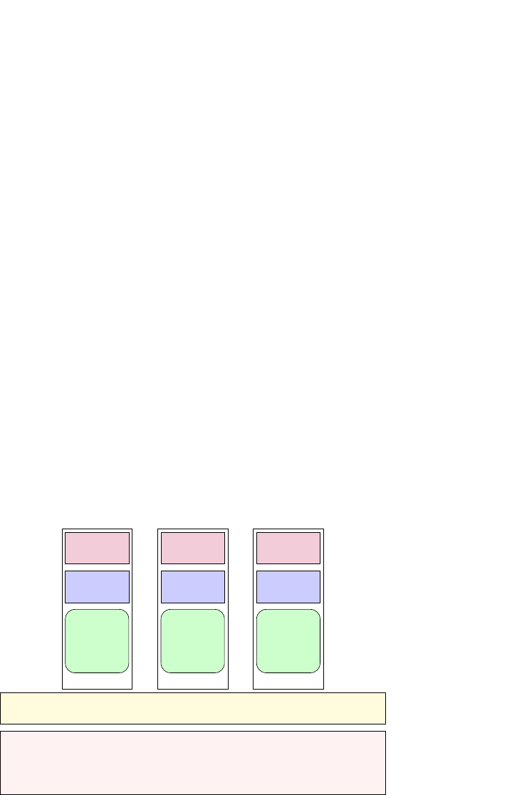
285
and distributed contexts, due to the metadata updates and consistency that are required. Parallel
frameworks oen layer custom distributed le systems on top of per-node le systems, for instance,
HDFS for Hadoop.
Global-scale distributed data systems are oen key-value stores, such as etcd or mongodb, which
feature replicaon and eventual consistency to migate latencies in wide area networks. Object
stores, such as Minio and Ceph, allow binary blobs to be stored at known locaons (perhaps web
addresses) with associated access controls and other metadata.
11.4 Virtualizaon and containerizaon
Ulity compung implies general compute resource is situated in the cloud. Users simply rent CPU
me on virtual servers they can provision on-demand.
Virtualizaon enables mulple virtual machines (VMs) to be hosted and isolated from each other
on a single physical node. The hypervisor layer mulplexes guest VMs on top of the host machine.
Figure 11.3 presents the concepts of virtualizaon as a schemac diagram. This approach is crucial
for infrastructure service providers to support exible deployment and resource overprovisioning.
It is possible to migrate a VM to another physical node if service levels are not sucient. Modern
processors have extensions to support virtualizaon navely. These include extra privilege levels and
an addional layer of indirecon in memory management. Linux supports hardware virtualizaon with
the Kernel-based Virtual Machine (KVM), which acts as a hypervisor layer. Virtual machine soware
that runs on top of KVM includes the QEMU full system emulator. This allows a disnct guest OS,
possibly compiled for a dierent processor architecture, to execute on top of the Linux host OS.
Figure 11.3: Schemac diagram for virtualizaon, showing that an app actually runs on top of two kernels (in guest and host OS respecvely).
There is an alternave approach: unlike fully-edged virtualizaon where each VM runs a disnct
guest OS, Linux containers enable lightweight isolaon of processes that share a common host OS
i
i
“chapter” — 2019/8/13 — 21:02 — page 3 — #3
i
i
i
i
i
i
Host OS
Hypervisor
Guest OS Guest OSGuest OS
libs
app
libs
app
libs
app
Virtual Machine Virtual Machine Virtual Machine
Chapter 11 | Advanced topics
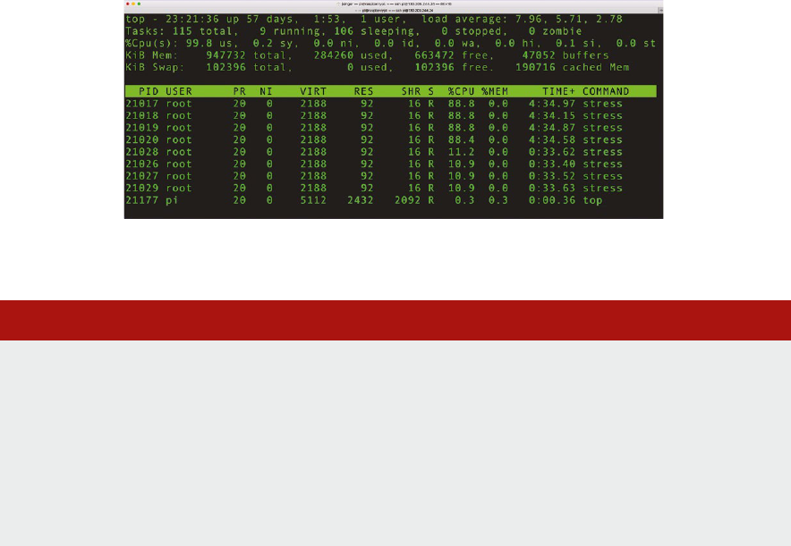
Operang Systems Foundaons with Linux on the Raspberry Pi
286
kernel. While containers lack the exibility of heavyweight virtualizaon, they are potenally much
more ecient. For this reason, containerizaon is popular for use cases requiring rapid deployment
mes such as DevOps, cloud systems, and serverless compung. A user wants to spin up a relevant
applicaon service with minimal latency. Tools like Docker enable services to be specied and
composed declaravely as scripts, then prebuilt images can match these scripts. This avoids lengthy
conguraon and build mes, enabling services to come up quickly.
Linux kernel facilies such as control groups (cgroups) enable containerizaon. Key concepts are
namespace isolaon and resource liming. Sets of processes can be collected together into a cgroup
and controlled as a unit. The bash lisng below illustrates how to exercise this control, and Figure 11.4
shows the outcome on a typical quad-core Raspberry Pi node.
Figure 11.4: CPU usage from top command, showing how Linux distributes CPU resource based on cgroups conguraon.
Lisng 11.4.1: Using cgroups to limit CPU resource Bash
1 sudo apt-get install stress # tool for CPU stress-testing
2 sudo apt-get install cgroup-tools # utils for cgroups
3 sudo cgcreate -g cpu:morecpu
4 sudo cgcreate -g cpu:lesscpu
5 cgget -r cpu.shares morecpu # default is 1024
6 sudo cgset -r cpu.shares=128 lesscpu # limit CPU usage
7 # now run some stress code in dierent control groups
8 sudo cgexec -g cpu:lesscpu stress --cpu 4 &
9 sudo cgexec -g cpu:morecpu stress --cpu 4 &
10 top # to see the CPU usage
11 sudo killall stress # to stop the stress jobs
Process sandboxes support throw-away execuon. Processes may be run once; then, their side-eects
may be isolated and discarded. In this sense, Linux containers are a progression of earlier Unix chroot
and BSD jail concepts. User-friendly conguraon tools like Docker have massively popularized
containerizaon.
The growth in the ulity compung market requires greater levels of resource awareness in the
underlying system. In parcular, the OS needs to support three key acvies:

287
1. Predicng: The OS must esmate ahead-of-me how long user tasks will take to complete and
which resources they will need. This is useful for ecient scheduling.
2. Accounng: The OS must keep track of precisely which resources are used by each applicaon.
This depends on low-level tools like perf, alongside higher-level applicaon-specic metrics such
as a number of database queries. This is essenal for billing users accurately for their workloads.
3. Constraining: The OS must allow certain sets of acons for each applicaon. Similar to sandboxing,
there are constraints on the applicaon behavior. Oen the constraints are expressed as a blacklist
of disallowed acons; this is generally how smartphone apps are executed. On the other hand, the
constraints could be expressed as a whitelist of allowable acons; this might be supported by a
capability-based system. CPU usage constraints, as outlined above, rely on quantave thresholds
that must be enforced by the kernel.
11.5 Security
In this secon, we discuss two recently discovered types of exploits that make use of aws in the
hardware to compromise the system. Appreciang these exploits requires knowledge of hardware
architecture (DRAM, cache, TLB, MMU, DMA), the memory subsystem, memory organizaon
(paging), and memory protecon. Therefore studying these exploits is a very good way to assess your
understanding of concepts covered in the book.
Figure 11.5: Logos for the Rampage exploit and Guardion migaon.
11.5.1 Rowhammer, Rampage, Throwhammer, and Nethammer
The original Rowhammer exploit makes use of a vulnerability in modern DRAM, in parcular, DDR3
and DDR4 SDRAM. Essenally, in such DRAMs, there is a non-zero probability of ipping a bit in a
given row by alternated accesses to the adjacent rows [4]. The actual exploit uses this aw by causing
permission bits to be ipped in a page table entry (PTE) that causes the PTE to point to a physical
page containing a page table of the aacking process. That process thereby gets read-write access to
one of its own page tables, and hence to the enre physical memory. A very good explanaon is given
in the original blog post by Mark Seaborn. You can also test if your own computer is vulnerable.
Several variants of this exploit have been developed: Rowhammer.js which uses hps://github.com/
IAIK/rowhammerjs [5], Rampage, which uses the Android DMA buer management API to induce
Chapter 11 | Advanced topics

Operang Systems Foundaons with Linux on the Raspberry Pi
288
the bit ips [6], and building on this hps://vusec.net/projects/throwhammer, which exploits remote
direct memory access (RDMA) [7] and Nethammer [8], which uses only a specially craed packet
stream. Neither of these exploits requires the aacker to run code on the target machine. All of the
cited papers also discuss migaon strategies against the exploits.
The DRAM on the Raspberry Pi board is DDR2, which is generally not vulnerable to Rowhammer-type
exploits.
11.5.2 Spectre, Meltdown, Foreshadow
A modern OS has memory protecon mechanisms which stop a process from accessing data
belonging to another user, and also stop user processes from accessing kernel memory. Speculave
execuon aacks exploit the fact that a CPU will already start accessing data before it knows if it is
allowed to, i.e., while the memory protecon check is in progress. In theory, this is permissible because
the results of this speculave execuon should be protected at the hardware level. If a process does
not have the right privilege, it is not allowed to access this data, and the data is discarded.
However, the protected data is stored in the cache regardless of the privilege of the process. Cache
memory can be accessed more quickly than regular memory. The aacker process can try to access
memory locaons to test if the data there has been cached, by ming the access. This is known as
a side-channel aack. Both Spectre and Meltdown, and also the more recent Foreshadow exploit,
work by combining speculave execuon and a cache side-channel aack.
Meltdown [9] gives a user process read access to kernel memory. The migaon in Linux is
a fundamental change to how memory is managed: as explained in Chapter 6, Linux normally maps
kernel memory into a poron of the user address space for each process. On systems vulnerable to
the Meltdown exploit, this allows the aacker process to read from the kernel memory. The soluon
is called kernel page-table isolaon (KPTI).
Spectre [10] is a more complex exploit, harder to execute, but also harder to migate against.
There are two variants: one ("bounds-check bypass", CVE-2017-5753) depends on the existence of
a vulnerable code sequence that is conveniently accessible from user space; the other ("branch target
injecon", CVE-2017-5715) depends on poisoning the processor’s branch-predicon mechanism so
that indirect jumps will under speculave execuon be redirected to an aacker-chosen locaon.
The migaon strategies are discussed in a post on LWN.
Finally, Foreshadow [11] (or L1 Terminal Fault) is the name for three speculave execuon
vulnerabilies that aect Intel processors. Foreshadow exploits a vulnerability in Intel’s SGX (Soware
Guard Extensions) technology. SGX creates a ‘secure enclave’ in which users can provide secure
soware code that will run without being observed by even the operang system. SGX protects
Meltdown and Spectre; however, Foreshadow manages to circumvent this protecon. A good
explanaon of the exploit is given by Jon Masters, chief ARM architect at Red Hat.
The Arm processor on the Raspberry Pi board is not suscepble to these speculave execuon aacks
as it does not perform speculave execuon.
289
Figure 11.6: Logos for the Meltdown and Spectre exploits—it seems that eye-catching graphics are compulsory for OS security violaons.
11.6 Vericaon and cercaon
Formal vericaon techniques use mathemacal models and proofs to provide guarantees about the
properes and behavior of systems. This is essenal as soware grows in size and complexity, and as
it becomes the essenal foundaon of our everyday societal interacons. Many industrial sectors are
establishing cered requirements for soware to be veried formally, e.g., ISO 26262 for automove
vehicles and DO-178C for aerospace. Since the OS is a crical part of the soware stack, it will
become increasingly necessary to apply vericaon techniques to sets of OS components.
Microso pioneered veried components for the Windows OS with its device driver vericaon
program. Poor quality, third-party device drivers running in privileged mode can compromise kernel
data structures and invariants, oen resulng in the ‘blue screen of death,’ see Figure 11.7. This is
the Windows equivalent of the Unix kernel panic. At one point, bugs in device drivers caused 85% of
system crashes in Windows XP. [12]
Figure 11.7: Blue screen of death in Windows XP (le) and Windows 10 (right) — since the driver vericaon program, such blue screens are much less
common. Photo by author.
The SLAM project blends ideas from stac analysis, model checking, and theorem proving [13]. The
key tool is the Stac Driver Verier (SDV) which analyzes C source code, typically a device driver
implementaon comprising thousands of lines of code, to check it respects a set of hard-coded rules
that encapsulate legal interacons with the Windows kernel.
Chapter 11 | Advanced topics
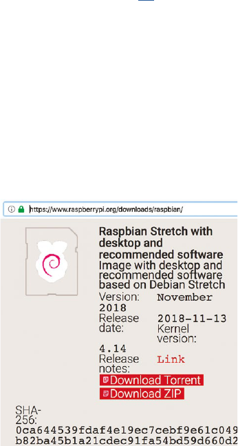
Operang Systems Foundaons with Linux on the Raspberry Pi
290
The SDV simplies input C code by converng it to an abstract boolean program, retaining the
original control ow but encoding all relevant program state as boolean variables. This abstract
program is executed symbolically to idenfy and report kernel API rule violaons. An example rule
species that locks should be acquired then subsequently released in strict sequence. The collecon
of pre-packaged API rules is harvested from previously idened error reports and Windows driver
documentaon. Empirical evidence shows the SDV approach has signicantly reduced bugs in
Windows device drivers.
When modern OS soware is built-in high-level languages such as C# and Rust, it is feasible to
perform stac analysis directly on the source code, to provide guarantees about memory safety and
data race freedom, for instance. Such guarantees may be composed to generate high-level OS safety
properes.
The seL4 project is a fully veried microkernel system [14]. The OS consists of small independent
components with clearly dened communicaon channels. Minimal funconality is provided in veried
microkernel, which is implemented in 10K lines of code, mostly C with some assembler. Properes
include access control guarantees, memory safety, and system call terminaon. Generally, there is
proof that the C source code matches the high-level abstract specicaon of the system. These kinds
of proofs are extremely expensive, in terms of expert human eort, to construct.
Cercaon involves mechanisms to guarantee the integrity of executable code. Cryptographic
hashes, such as MD5 and SHA1, are used to check a le has not been modied. For instance, when
you download a Raspbian SD card image from the Raspberry Pi website or a mirror, it is possible to
check the published SHA-256 hash of the le to guarantee its authencity, see Figure 11.8.
Figure 11.8: OS image hash is published alongside the download link to ensure authencity.
A signed executable ensures provenance as well as integrity. Using public key infrastructure, a code
distributor can sign the executable le or a hash of the le with their private key. A potenal user
can check the signature and the hash, to be sure the code is from an appropriate source and has not
been modied. Linux ulies like elfsign or the Integrity Measurement Architecture support digital

291
signatures for executable les. Hardware support, such as Arm TrustZone, is required for secure code
cercaon. In parcular, it is necessary to check the rmware and boot loader to ensure that only
cered code is able to run on the system.
Reproducibility is a key goal in modern systems. This is important for scienc experiments, for
debugging, for ensuring compability in a highly eclecc system of soware components. Declarave
scripng languages, like those provided by Nix or Puppet, enable systems to be congured easily to a
common standard. This is ideal for DevOps scenarios. The Nix package manager keeps track of all data
and code dependencies required to build each executable, via a cryptographic hash. This is encoded
directly in the path for the executable, e.g. /nix/store/a9i0a06gcs8w9fj9nghsl0b6vvqpzpi4-
bash-4.4-p23 which means mulple versions of an applicaon can co-exist in the same system,
and be managed easily with congurable proles. System administrators never need to ‘overwrite’ an
old applicaon or library when they upgrade to a new version, which makes compability and rollback
much easier.
Lisng 11.6.1: Example nix docker session Bash
1 # check out https://nixos.org/nix/manual/
2 # for more details
3 docker pull nixos/nix
4 docker run -it nixos/nix
5 nix-env -qa
6 nix-build '<nixpkgs>' -A hello
7 nix-shell '<nixpkgs>' -A hello
8 ./result/bin/hello
9 ls -l ./result
11.7 Recongurability
As compung plaorms become more exible, incorporang technology such as FPGA accelerators,
the OS must support on-the-y reconguraon. Similarly, in cloud compung contexts, the resources
available to a VM may change as the guest OS is migrated to dierent virtual servers with a range of
hardware opons. Even a commodity CPU on a laptop can be congured to operate at dierent clock
frequencies, trading o compute performance and power consumpon.
Presently, Linux supports dynamic reconguraon with a range of heurisc policies for parcular
resources. For instance, there is a CPU frequency governor that controls processor clock frequency
depending on current resource usage. Various research projects have explored the potenal for
machine learning to enable automac runme tuning of OS parameters. To date, there is no machine
learning component embedded in a mainstream OS kernel. Self-tuning systems based on machine
learning may arrive soon, although they would not be compliant with current domain-specic
cercaon, e.g., in the automove or aerospace sectors.
There is an accelerang trend to move OS components into user space. We introduced the noon
of a le system in user space (FUSE) in Chapter 9. Networking in user space is also supported, with
frameworks like the Data Plane Development Kit (DPDK) that support accelerated, customized
packet processing in user applicaon code. This exibility enables techniques like soware-dened
Chapter 11 | Advanced topics
Operang Systems Foundaons with Linux on the Raspberry Pi
292
networking and network funcon virtualizaon. Eecvely, the network stack can be recongured at
runme in soware.
In theory, as the Linux kernel transfers these tradional OS responsibilies to user space code, its
architecture increasingly resembles a micro-kernel OS. The historical cricism of Linux was that it was
too monolithic to scale and survive, see Figure 11.9. Torvalds addressed these cricisms directly at the
me, and reected on his design principles at a later date [15].
Figure 11.9: Part of the famous ‘Linux is obsolete’ debate focused on its non-microkernel architecture. Cartoons by Lovisa Sundin.
11.8 Linux development roadmap
There is no formal roadmap for Linux kernel development. There are a number of release candidates
with experimental features, some of which will be incorporated in future stable releases.
Check hps://kernel.org for the latest details. The Linux Weekly News service keeps track of ongoing
changes to the kernel, see hps://lwn.net/Kernel/
i
i
“chapter” — 2019/8/13 — 21:02 — page 9 — #9
i
i
i
i
i
i
Andrew Tanenbaum
Subject: LINUX is obsolete
MINIX is a microkernel-based system.
The file system and memory management
are separate processes, running outside
the kernel. The I/O drivers are also
separate processes (in the kernel, but
only because the brain-dead nature of
the Intel CPUs makes that difficult to
do otherwise). LINUX is a monolithic
style system. This is a giant step back
into the 1970s. That is like taking an
existing, working C program and rewriting
it in BASIC. To me, writing a monolithic
system in 1991 is a truly poor idea.
Tanenbaum’s criticism of the Linux architecture on Usenet (29 Jan 1992)
>1. MICROKERNEL VS MONOLITHIC SYSTEM
True, linux is monolithic, and I agree
that microkernels are nicer. With a less
argumentative subject, I’d probably have
agreed with most of what you said. From
a theoretical (and aesthetical) standpoint
linux loses [sic].
>MINIX is a microkernel-based system.
>[deleted, but not so that
>you miss the point ]
>LINUX is a monolithic style system.
If this was the only criterion for
the "goodness" of a kernel, you’d be
right...
Excerpt of Torvalds’ response on Usenet (29 Jan 1992)
Linus Torvalds
Andrew Tanenbaum
i
i
“chapter” — 2019/8/13 — 21:02 — page 9 — #9
i
i
i
i
i
i
Andrew Tanenbaum
Subject: LINUX is obsolete
MINIX is a microkernel-based system.
The file system and memory management
are separate processes, running outside
the kernel. The I/O drivers are also
separate processes (in the kernel, but
only because the brain-dead nature of
the Intel CPUs makes that difficult to
do otherwise). LINUX is a monolithic
style system. This is a giant step back
into the 1970s. That is like taking an
existing, working C program and rewriting
it in BASIC. To me, writing a monolithic
system in 1991 is a truly poor idea.
Tanenbaum’s criticism of the Linux architecture on Usenet (29 Jan 1992)
>1. MICROKERNEL VS MONOLITHIC SYSTEM
True, linux is monolithic, and I agree
that microkernels are nicer. With a less
argumentative subject, I’d probably have
agreed with most of what you said. From
a theoretical (and aesthetical) standpoint
linux loses [sic].
>MINIX is a microkernel-based system.
>[deleted, but not so that
>you miss the point ]
>LINUX is a monolithic style system.
If this was the only criterion for
the "goodness" of a kernel, you’d be
right...
Excerpt of Torvalds’ response on Usenet (29 Jan 1992)
Linus Torvalds
Linus Torvalds

293
11.9 Further reading
Throughout this chapter, we have given a avor of contemporary trends in OS development and
deployment. Some of these issues have an immediate impact on Linux; others may aect the plaorm
over the next decade.
The annual workshop on Hot Topics in Operang Systems (HotOS) is an excellent venue for OS future
studies and speculaon. If you are interested in OS research and development, consult recent years’
proceedings of this event, which should be available online.
11.10 Exercises and quesons
11.10.1 Make a minimal kernel
Congure and build a custom Linux kernel for your Raspberry Pi. How small a kernel image can
you create?
11.10.2 Verify important properes
Veried soware systems provide formal guarantees about their properes and behavior. Suggest
some properes you might want to prove about components of an OS.
11.10.3 Commercial comparison
Much of the popularity of Linux could be aributed to the fact it is free, open-source, soware (FOSS).
Compare Linux with a mainstream OS that is not FOSS. Can you idenfy dierences, and explain why
they might occur? Is there a dierent emphasis on developing new features?
11.10.4 For or against cercaon
Soware cercaon has a number of advantages and disadvantages, which must be carefully
assessed. Draw up a debate card, lisng the pros and cons of OS cercaon. This could form the
basis for a group discussion with your peers.
11.10.5 Devolved decisions
The modern Linux kernel abdicates responsibility for certain policies to user space, e.g., for le systems
(with FUSE) and networking (with DPDK). Discuss other services that might be transferred from the
kernel to user space. System logging is one candidate.
11.10.6 Underclock, overclock
It is possible to modify the conguraon of your Raspberry Pi board to change the CPU clock
frequency. Find the line specifying arm_freq = 1200 in your /boot/cong.txt and modify this. The
frequency is specied as an integer, denong MHz. There are other frequencies you can change, such
as those for GPU and memory. Check online documentaon for details, and note that some sengs
may void your warranty.
You can invesgate how frequency and power trade-o, by monitoring your Raspberry Pi power
consumpon when you run CPU-intensive applicaons (perhaps the stress ulity). You will need to
use an external USB digital mulmeter or power monitor. Produce a graph to show the relaonship
between frequency in MHz and power in W.
Chapter 11 | Advanced topics

Operang Systems Foundaons with Linux on the Raspberry Pi
294
References
[1] L. A. Barroso, U. Hölzle, and P. Ranganathan, The Datacenter as a Computer: Designing Warehouse-Scale Machines, 3rd ed.
Morgan Claypool, 2018.
[2] M. Maas, K. Asanovic ́, T. Harris, and J. Kubiatowicz, “Taurus: A holisc language runme system for coordinang distributed
managed-language applicaons,” in Proceedings of the Twenty-First Internaonal Conference on Architectural Support for
Programming Languages and Operang Systems, 2016, pp. 457–471.
[3] E. S. Raymond, Plan 9: The Way the Future Was. Addison Wesley, 2003, hp://catb.org/~esr/wrings/taoup/html/plan9.html
[4] Y. Kim, R. Daly, J. Kim, C. Fallin, J. H. Lee, D. Lee, C. Wilkerson, K. Lai, and O. Mutlu, “Flipping bits in memory without
accessing them: An experimental study of DRAM disturbance errors,” in ACM SIGARCH Computer Architecture News, vol. 42,
no. 3, 2014, pp. 361–372.
[5] D. Gruss, C. Maurice, and S. Mangard, “Rowhammer.js: A remote soware-induced fault aack in Javascript,” in Internaonal
Conference on Detecon of Intrusions and Malware, and Vulnerability Assessment. Springer, 2016, pp. 300–321.
[6] V. Van Der Veen, Y. Fratantonio, M. Lindorfer, D. Gruss, C. Maurice, G. Vigna, H. Bos, K. Razavi, and C. Giurida, “Drammer:
Determinisc Rowhammer aacks on mobile plaorms,” in Proceedings of the 2016 ACM SIGSAC conference on computer and
communicaons security, 2016, pp. 1675–1689.
[7] A. Tatar, R. Krishnan, E. Athanasopoulos, C. Giurida, H. Bos, and K. Razavi, “Throwhammer: Rowhammer aacks over the
network and defenses,” in 2018 USENIX Annual Technical Conference, 2018.
[8] M. Lipp, M. T. Aga, M. Schwarz, D. Gruss, C. Maurice, L. Raab, and L. Lamster, “Nethammer: Inducing Rowhammer faults
through network requests,” arXiv preprint arXiv:1805.04956, 2018.
[9] M. Lipp, M. Schwarz, D. Gruss, T. Prescher, W. Haas, A. Fogh, J. Horn, S. Mangard, P. Kocher, D. Genkin et al., “Meltdown:
Reading kernel memory from user space,” in 27th USENIX Security Symposium, 2018, pp. 973–990.
[10] P.Kocher, D.Genkin, D.Gruss, W.Haas, M.Hamburg, M.Lipp, S.Mangard, T.Prescher, M.Schwarz, and Y. Yarom, “Spectre
aacks: Exploing speculave execuon,” arXiv preprint arXiv:1801.01203, 2018.
[11] J.VanBulck, M.Minkin, O.Weisse, D.Genkin, B.Kasikci, F.Piessens, M.Silberstein, T.F.Wenisch, Y. Yarom, and R. Strackx,
“Foreshadow: Extracng the keys to the Intel SGX kingdom with transient out-of-order execuon,” in 27th USENIX Security
Symposium, 2018, pp. 991–1008.
[12] T.Ball, E.Bounimova, B.Cook, V.Levin, J.Lichtenberg, C.McGarvey, B.Ondrusek, S.K.Rajamani, and A. Ustuner, “Thorough
stac analysis of device drivers,” ACM SIGOPS Operang Systems Review, vol. 40, no. 4, pp. 73–85, 2006.
[13] T.Ball, B.Cook, V.Levin, and S.K.Rajamani, “SLAM and Stac Driver Verier: Technology transfer of formal methods inside
Microso,” Tech. Rep. MSR-TR-2004-08, 2004, hps://www.microso.com/en-us/research/wp-content/uploads/2016/02/tr-
2004-08.pdf

295
[14] G.Klein, J.Andronick, K.Elphinstone, G.Heiser, D.Cock, P.Derrin, D.Elkaduwe, K.Engelhardt, R.Kolanski, M. Norrish, T. Sewell,
H. Tuch, and S. Winwood, “seL4: Formal vericaon of an operang-system kernel,” Communicaons of the ACM, vol. 53, no. 6,
pp. 107–115, Jun. 2010.
[15] L. Torvalds, The Linux Edge. O’Reilly, 1999, hp://www.oreilly.com/openbook/opensources/book/linus.html
Chapter 11 | Advanced topics

Operang Systems Foundaons with Linux on the Raspberry Pi
296
Address space A set of discrete memory addresses. The physical address space is the set
of all of the memory in a computer system, including the system memory
(DRAM) as well as the I/O devices and other peripherals such as disks.
Applicaon binary
interface (ABI)
The specicaons to which an executable must conform in order to
execute in a specic execuon environment.
Arithmec logic unit
(ALU)
The part of a processor that performs computaons.
Assembly language A low-level programming language with a very strong correspondence
between the program’s statements and the architecture’s machine code
instrucons, used as a target by compilers for higher-level languages.
Atomic operaon An operaon which is guaranteed to be isolated from interrupts,
signals, concurrent processes, and threads.
Boong The process of starng up a computer system and pung it in a state
so that it can be used.
Cache A small but fast memory used to limit the me spent by the CPU in
waing for main memory access. For every memory read operaon,
rst the processor checks if the data is present in the cache, and
if so (cache hit) it uses that data rather than accessing the DRAM.
Otherwise (cache miss) it will fetch the data from memory and store
it in the cache.
Cache coherency In a mulcore computer system with mulple caches, cache
coherency (or cache coherence or) is the mechanism that ensures that
changes in data are propagated throughout the memory system in a
mely fashion so that all the caches of a resource have the same data.
Clock ck Informal synonym for _clock cycle_, the me between two
consecuve rising (posive) edges of the system clock signal.
Complex instrucon set
compung (CISC)
A CPU with a large set of complex and specialized instrucons rather
a small set of simple and general instrucons. The typical example is
the x86 architecture.
Concurrency The fact that more than one task is running concurrently (at the same
me) on the system. In other words, concurrency is a property of
the workload rather than the system, provided that the system has
support for running more than one task at the same me. In pracce,
one of the key reasons to have an OS is to support concurrency
through scheduling of tasks on a single shared CPU.
Glossary of terms

297
Crical secon A secon of a program which cannot be executed by more than one
process or thread at the same me. Crical secons typically access
a shared resource and require synchronizaon primives such as
mutual exclusion locks to funcon correctly.
Deadlock The state in which each process in a group of communicang process is
waing for a message from the other process in order to proceed with
an acon. Alternavely, in a group of processes with shared resources,
there will be deadlock if each process is waing for another process to
release the resource that it needs to proceed with the acon.
Direct memory access
(DMA)
A mechanism that allows peripherals to transfer data directly into
the main memory without going through the processor registers.
In Arm systems, the DMA controller unit is typically a peripheral.
DRAM Dynamic random-access memory, high-density memory, slower than
SRAM. It is typically used as the main memory in a computer system.
A DRAM cell is typically a small capacitor. As the charge leaks, it
needs to be periodically refreshed.
Endianness The sequenal order in which bytes are arranged into words when
stored in memory or when transmied over digital links. There are
two incompable formats in common use, called big-endian and
lile-endian. In big-endian format, the most signicant byte (the byte
containing the most signicant bit) is stored at the lowest address.
Lile-endian format reverses this order.
Everything is a le A key concept in Linux and other UNIX-like operang systems.
It does not mean that all objects in Linux are les as dened above,
but rather that Linux prefers to treat all objects from which the
OS can read data or to which it can write data using a consistent
interface. So it might be more accurate to say, "everything is a stream
of bytes." Linux uses the concept of a le descriptor, an abstract
handle used to access an input/output resource (of which a le
is just one type). So one can also say that in Linux, “everything is
a le descriptor.”
File A named set of related data that is presented to the user as a single,
conguous block of informaon, and that is kept in persistent storage.
File system A system for the logical organizaon of data. The purpose of most le
systems is to provide the le and directory (folder) abstracons. A le
system not only allows to store informaon in the form of les organized
in directories but also informaon about the permissions of usages for
les and directories, as well as mestamp informaon. The informaon
in a le system is typically organized as a hierarchical tree of directories,
and the directory at the root of the tree is called the root directory.
Glossary of terms

Operang Systems Foundaons with Linux on the Raspberry Pi
298
Hypervisor A program, rmware, or hardware system that creates and runs virtual
machines.
Instrucon A computer program consists of a series of instrucons. Each
instrucon determines how the processor interacts with the system
through the address space.
Interrupt A signal sent to the processor by hardware (peripherals) or soware
indicang an event that needs immediate aenon. The acon of
sending the signal is called an interrupt request (IRQ).
Kernel The program that is the core of an operang system, with complete
control over everything in the system. It is usually one of the rst
programs loaded when boong the system (aer the bootloader).
It handles the rest of startup and inializaon as well as requests for
system services from other processes.
Memory The hardware that stores informaon for immediate use in
a computer, typically SRAM or DRAM.
Memory management unit
(MMU)
A computer system hardware component which manages memory
access control and memory address translaon, in parcular, the
translaon of virtual memory addresses to physical addresses.
Memory address An unsigned integer value used as the idener for a word of data
stored in memory.
MIPS for the masses The slogan of the original Arm design team, which aimed to create
a cheap but powerful processor that would provide lots of processing
power ("MIPS" means Millions of Instrucons Per Second) for a price
that everybody could aord.
Mnemonic An abbreviaon for an operaon. Assembly language uses
mnemonics to represent each low-level machine instrucon or
opcode, typically also each architectural register, ag, etc. Also the
surname of the eponymous character in William Gibson’s novella
"Johnny Mnemonic" (1981).
MPI (Message passing
interface)
An API specicaon designed for high-performance compung.
It provides a distributed memory model for parallel programming.
Its main targets have been clusters and mulprocessor machines, but
recently also manycore system. The message passing model means
that tasks do not share any memory. Instead, every task has its own
private memory, and any communicaon between tasks is via the
exchange of messages.
Glossary of terms

299
Mounng The operaon performed by the kernel to provide access to a le system.
Mounng a le system aaches that le system to a directory (mount
point) and makes it available to the system. The root le system is always
mounted. Any other le system can be connected or disconnected from
the root le system at any point in the directory tree.
Multasking The concurrent execuon of mulple tasks (also known as processes)
over a certain period of me.
Network interface
controller (NIC)
Also known as a network interface card or network adapter,
is a computer hardware component that connects a computer to
a computer network.
Networking The interacon of a computer system with other computer systems
using an intermediate communicaon infrastructure.
Opcode An opcode or operaon code is the part of a machine language
instrucon that species the operaon to be performed. Most
instrucons also specify the data to be processed in the form of
operands.
OpenCL An open standard for parallel compung on heterogeneous architectures.
OpenMP A standard for shared-memory parallel programming. It is based on
a set of compiler direcves or pragmas, combined with a programming
API to specify parallel regions, data scope, synchronizaon, etc..
OpenMP is a portable parallel programming approach, and the
specicaon supports C, C++, and Fortran.
Operang system An operang system (OS) is a dedicated program that manages
the hardware and soware resources of a computer system and
provides common services for computer programs running on the
system. Modern operang systems keep track of resource usage
of tasks and use me-sharing to schedule tasks for ecient use of
the system.
Parallelism Parallel processing is a capability of a computer system.
Paron A disk can be divided into parons, which means that instead of
presenng as a single blob of data, it presents as several dierent
blobs. Parons a are logical rather than physical, and the informaon
about how the disk is paroned is stored in a paron table.
Peripheral A device connected to a computer, used to put informaon into and
get informaon out of the computer. "The Peripheral" is also the name
of a science con novel by William Gibson (2014).
Glossary of terms

Operang Systems Foundaons with Linux on the Raspberry Pi
300
Persistent storage Also known as non-volale storage is a type of storage that retains its
data even if the device is powered o. Examples are solid-state drives
(SSD), hard disks, and magnec tapes.
Polling The acon of periodically checking the state of a peripheral.
POSIX The Portable Operang System Interface (POSIX) is a family of IEEE
standards aimed at maintaining compability between operang
systems. POSIX denes the applicaon programming interface (API)
used by programs to interact with the operang system.
Preempon The act of temporarily interrupng a task being carried out by a
computer system (and in parcular a process running on a CPU),
without requiring the cooperaon of that task, and with the intenon
of resuming the task at a later me. Preempon is a key feature
of preempve multasking. The alternave approach where the
cooperaon of a task is needed is called cooperave multasking.
Process A process is a running program, i.e., the code for the program and
all system resources it uses. The concept of a process is used for the
separaon of code and resources. With this denion, a process can
consist of mulple threads.
Process control block
(PCB)
Also called Task Control Block (TCB). The operang system kernel
data structure, which contains the informaon needed to manage the
scheduling of a parcular process.
RAM Random-access memory. Data stored in RAM can be read or wrien in
almost the same amount of me irrespecve of the physical locaon
of data inside the memory. This as opposed to other direct-access data
storage media such as hard disks, CDs, DVDs, and magnec tapes.
Reduced instrucon set
compung (RISC)
A CPU with a small set of simple and general instrucons, rather than
a large set of complex and specialized instrucons. Arm processors
have a RISC architecture.
Register le An array of words called registers, typically implemented as SRAM
memory and part of the CPU.
Root user In Linux and other Unix-like computer OSes, root is the convenonal
name of the user who has all rights or permissions (to all les and
programs) in all modes (single- or mul-user). Alternave names
include superuser and administrator. In Linux, the actual name of the
account is not the determining factor.
Scheduling The mechanism used by the operang system kernel to allocate CPU
me to tasks.
Glossary of terms

301
SIMD (Single instrucon
mulple data)
A type of parallel computaon where mulple processing elements
perform the same operaon on mulple data points simultaneously.
SRAM Stac random-access memory, lower-density memory, faster than
DRAM. It is typically used for cache memory in a computer system.
An SRAM cell is a latch, so it retains its value as long as the device is
powered on, without the need for refreshing.
Symmetric
mulprocessing (SMP)
An operaonal model for mulcore computer systems where two or
more idencal cores are connected to a single, shared main memory,
have full access to all input and output devices, and are controlled by
a single operang system instance that treats all processors equally,
reserving none for special purposes. Most modern mulcore systems
use an SMP architecture.
System clock A counter of the me elapsed since some arbitrary starng date
called the epoch. Linux and other POSIX-compliant systems encode
system me as the number of seconds elapsed since the start of
the Unix epoch at 1 January 1970 00.00.00 UT, with excepons for
leap seconds.
System state The set of all informaon in a system that the system remembers
between events or user interacons.
System-on-chip (SoC) Also called system-on-a-chip, an IC (integrated circuit) that integrates
all components of a computer system. These components typically
include a CPU, memory, I/O ports, and secondary storage, combined
on a single chip.
Task A unit of execuon or a unit of work on a computer system. The term
is somewhat less strictly dened and usually relates to scheduling.
Thread Mulple concurrent tasks execung within a single process are called
threads of execuon. The threads of a process share its resources.
For a process with a single thread of execuon, the terms task and
process are oen used interchangeably.
Timer A specialized type of clock used for measuring specic me intervals.
Translaon look-aside
buer (TLB)
A special type of cache which stores recent translaons of virtual
memory to physical memory. It is part of the MMU.
User In general, a user is a person who ulizes a computer system.
However, in the context of an operang system, the term user is used
more broadly to idenfy the ownership of processes and resources.
Therefore a user does not need to be a person.
Glossary of terms

Operang Systems Foundaons with Linux on the Raspberry Pi
302
Virtual machine A program which emulates a computer system. Virtual machines are
based on computer architectures and provide the funconality of a
physical computer. Modern computer systems provide hardware support
for deployment of Virtual Machines (virtualizaon) through hypervisors.
Word A xed-size, conguous array of bits used by a given processor
design. A word is a xed-sized piece of data handled as a unit by the
instrucon set or the hardware of the processor. The number of bits
in a word (also called word size, word width, or word length) is a key
characterisc for any specic processor architecture. Typically, a word
consists of a number of bytes (a sequence of 8 bits), which are stored
either in lile-endian or big-endian format (see endianness). The most
common word sizes for modern processors are 64 and 32 bits, but
processors with 8 or 16-bit word size are sll used for embedded
systems.
Glossary of terms

303
Operang Systems Foundaons with Linux on the Raspberry Pi

Operang Systems Foundaons with Linux on the Raspberry Pi
304
Index
AArch32 6, 54-55
AArch64 50, 54-55, 57, 94
Accelerator Coherency Port 64
Accept 255, 259
Acon 2, 4-6
Address map
space
space layout, see Address map
space layout randomizaon
3-4, 61-63, 129
6, 23, 61-63, 128-131, 148, 296
149
Advanced high-performance bus 50
ALU, see Arithmec logic unit
Applicaon binary interface 94, 296
Arithmec Logic Unit 8, 296
Arm Cortex A53 50, 53-61
Arm Cortex M0+ 50-52
Armv6-M 51-52
Armv8-A 50, 53-55
Assembly language 8, 296
Associave 15, 58, 185
Atomic 165-169, 222, 296
Big-endian 257, 297
Binary tree 185
Bind 255, 258-259
Bitmap 165-167, 234
Block device 204
Blocking IO 207
Boot process (see also Boong)
sequence (see also Boong)
36-37, 183
36
Boong 36, 183, 296
Bootloader 32, 36
Branch 7, 9
Buer cache 142, 242
Cache
coherency
15-18, 59-61, 127, 142, 296
61, 64, 296
Character device 203-204
Chgrp 35, 225

305
Index
Chrt 111, 120
Clock processor clock
page replacement algorithm
system clock
cycle
ck
2, 13, 291
143-144
5, 301
5, 91
296
Completely fair scheduler 107
Complex instrucon set compung 50, 296
Concurrency 20, 158-161, 296
Connect 255, 260-261
Context switch 81-82
Control ow 12
Copy on write 72, 146-147
Core 49-50, 149, 159
Cortex, see Arm Cortex
Credenals 34-35, 225
Deadlock 161-162, 297
Demand paging 145
Device driver
tree
31, 38, 204, 253
32
Dijkstra 162-163
Directory 219-220, 231-233
Direct memory access 13-14, 63, 210, 297
DMA, see Direct memory access
Docker 244, 286
DRAM, see Dynamic random access memory
Dynamic shared object 95
Dynamic random access memory 3, 127, 287, 297
EABI 94-95
Earliest deadline rst 101, 112
Ethernet 206, 250, 253
Everything is a le 33, 218, 284, 297
Evict 15, 60, 144
Exclusive monitor 163-164
Exec 73, 275
Extended le system 233
Extents 236
Ext4 233-238

Operang Systems Foundaons with Linux on the Raspberry Pi
306
Index
FAT, see le allocaon table
Fetch-decode-execute cycle 8
File
allocaon table
system
218, 297
238-242
32-33, 218-220, 228-230, 297
Floang-point unit 55
Fork 71-74, 275
Fsck 243
Futex 174
Getsockopt 262
Gey 38
Groupadd 35
Heterogeneous mulprocessing 181
Host layers 251
HTTP 250
Hypervisor 56-57, 285, 298
IEEE 754-2008 55
Illegal instrucon 86-87
Init 34, 37-38, 77
Inializaon 37, 183
Inode 230-231
Insmod 39, 205
Instrucon
cycle
register
set
5-8, 298
8
9
50-51, 54
Interrupt
handler
request
service roune, see Interrupt handler
vector table
4, 209-211, 298
210-213
4, 13
13
Ioctl 207
IRQ, see Interrupt request
ISR, see Interrupt service roune
IVT, see Interrupt vector table
Journal 237
Kbuild 42

307
Index
Kernel Linux
OpenCL
module
space
31-32, 37-42, 76, 292, 298
192
39-42, 204
32
Kill 83
Large physical address extension 61, 133
LDREX 163-164
Least recently used 144
Link register 6, 12
Listen 255, 259
Lile-endian 257, 297
Load balancing 183-184
Logical address space 23
Login 38
LR, see Link register
MapReduce 185, 195
Media layers 251-252
Memory
address
barrier
management, see Memory
management unit
operaon ordering
protecon
protecon unit
126, 298
298
170-172
57, 129, 298
169
52, 152, 288
24, 52
Memset 259
MIPS for the masses 48, 298
Modprobe 39
MOESI 61
Monitor 163-164
MPI 190-191, 283, 298
Mprotect 152
Mutex 163, 174-177, 178
NEON (see also SIMD) 53
Nested vectored interrupt controller 51
Network adapter
interface controller
layer
protocol
250, 299
250, 299
252
253

Operang Systems Foundaons with Linux on the Raspberry Pi
308
Index
Networking 250-279, 299
Nice 102, 104, 119
Non-blocking IO 207
Non-preempve 96-100
Not recently used 143
Opcode 9, 299
OpenCL 191-194, 299
OpenMP 189-191, 299
OSI 251-252
Page cache
fault
table
table entry metadata
166
138-141
130-137
134
Parallelism 181-185, 189, 193, 195, 299
Paron 32, 299
PC, see Program counter
Peripheral 2, 299
Permissions 34-35, 225
Persistent storage (see also le system) 300
Physical address
address space
23, 128-130
3
Plan 9 284
Polling 209, 300
POSIX 42, 299
Preempon 96-100, 115-116, 300
Preempve 96-100, 102
Priories 98-99, 104-107, 119
Privileges 23, 34-35
Process, see Task (also see Thread)
control block
lifecycle
74-76, 300
70, 91-92
Program counter 6, 9
Programming model 158
Pthreads 186-189
RAM, see Random access memory
Random access memory 3, 126-127, 300
Raspberry Pi 36, 53

309
Index
RAM, see Random access memory
Random access memory 3, 126-127, 300
Raspberry Pi 36, 53
Read 256, 258, 262, 271
Read-modify-write 165
Recv 255, 261-262, 268, 271
Red-black tree 116-119
Reduced instrucon set compung 50, 300
Reducon 185
Register 6, 55, 300
Renice 119
Rmmod 39, 213
Root directory
user
33, 219
34, 300
Round-robin 21, 98
Scheduler 21, 31, 98, 184
Scheduling 21, 31, 43, 90-122, 184
Select 271-273, 275-276
Semaphore 159, 162-163, 175-179
Send 255, 261, 264, 268, 271
Sendto 255, 268, 271
Setsockopt 255, 262-265
SEV 183
Shared resource 158-160
Shortest job rst
remaining me rst
99
99
Signal handler 84
SIMD, see Single instrucon mulple data
Single instrucon mulple data 55, 182, 300
Socket 255-263, 265-268, 271
SP, see Stack pointer
Spin lock 173, 179
Stack
pointer
6, 11, 148
6, 11-12, 23, 52, 57
State 3
Stream socket 255-256, 261-262

Operang Systems Foundaons with Linux on the Raspberry Pi
310
Index
STREX 163-164
Subroune call 12-13
Superblock 229, 233-234
Supervisor 52
Swap cache
space
166
138
SWI 95, 210
Symmetric mulprocessing 164, 169, 183, 301
Synchronizaon 161, 163-165, 171-172, 177, 189-190, 194-195
Syscall 94-95
System state
mer
2-6, 301
21, 52
System-on-a-chip 36, 206, 301
Systemd 37-38
Tanenbaum 292
Task (see also Process)
scheduler
_struct
20-22, 90, 301
21
76, 102
TCP 252-253, 255, 264-267
TCP/IP 44, 250, 252-253
Thread
_info
31, 77, 101-102, 186, 301
76
Threading building blocks 194-195
Thumb 49, 51-52, 54
Time
slice
slicing
92-93, 140
21, 98
21
TLB, see Translaon look-aside buer
Torvalds 282, 292
Translaon look-aside buer 24, 58, 136, 301
Transport layer 254-255
UDP 253, 268-271
Ulimit 35, 221
Union le system 244
User
space
34, 301
20, 32
Useradd 35

311
Index
Virtual address space
memory
le system
128-129
127-130
75, 228-229
Wait 73-74
Waing (process state) 79-80, 92
Wilson 48
Working set 141
x86 50
YIELD 183
Zombie 80

Operang Systems Foundaons with Linux on the Raspberry Pi
312
Arm Educaon Media
Online Courses
Our online courses have been developed to help students learn about state-of-
the-art technologies from the Arm partner ecosystem. Each online course contains
10-14 modules, and each module comprises lecture slides with notes, interacve
quizzes, hands-on labs and lab soluons. The courses will give your students an
understanding of Arm architecture and the principles of soware and hardware
system design on Arm-based plaorms, skills essenal for today’s computer
engineering workplace.
Contact: [email protected]
Available now:
Ecient Embedded Systems Design and Programming
Rapid Embedded Systems Design and Programming
Digital Signal Processing
Internet of Things
Graphics and Mobile Gaming
System-on-Chip Design
Real-Time Operang Systems Design and Programming
Advanced System-on-Chip Design
Embedded Linux
Mechatronics and Robocs

313
Introducon to System-on-Chip Design
Online Courses
The Internet of Things promises devices endowed with processing, memory,
and communicaon capabilies. These processing nodes will be, in eect, simple
Systems-on-Chips (SoCs). They will need to be inexpensive, and able to operate
under stringent performance, power and area constraints.
The Introducon to System-on-Chip Design Online Course focuses on building
SoCs around Arm Cortex-M0 processors, which are perfectly suited for IoT
needs. Using FPGAs as prototyping plaorms, this course explores a typical SoC
development process: from creang high-level funconal specicaons to design,
implementaon, and tesng on real FPGA hardware using standard hardware
descripon and soware programming languages.
Discover more at www.armedumedia.com
Learning outcomes:
Knowledge and understanding of
Arm Cortex-M processor architectures
and Arm Cortex-M based SoCs
Design of Arm Cortex-M based SoCs in
a standard hardware descripon language
Low-level soware design for Arm Cortex-M
based SoCs and high-level applicaon
development
Intellectual
Ability to use and choose between dierent
techniques for digital system design and
capture
Ability to evaluate implementaon results
(e.g., speed, area, power) and correlate them
with the corresponding high-level design
and capture
Praccal
Ability to use commercial tools to develop
Arm Cortex-M based SoCs
Course Syllabus:
Prerequisites: Basics of hardware descripon
language (Verilog or VHDL), Basic C, and
assembly programming.
Modules
1. Introducon to Arm-based System-on-Chip
Design
2. The Arm Cortex-M0 Processor Architecture:
Part 1
3. The Arm Cortex-M0 Processor Architecture:
Part 2
4. AMBA3 AHB-Lite Bus Architecture
5. AHB SRAM Memory Controller
6. AHB VGA Peripheral
7. AHB UART Peripheral
8. Timer, GPIO, and 7-Segment Peripherals
9. Interrupt Mechanisms
10. Programming an SoC Using C Language
11. Arm CMSIS and Soware Drivers
12. Applicaon Programming Interface and
Final Applicaon
Operang Systems Foundaons with Linux on the Raspberry Pi

Operang Systems Foundaons with Linux on the Raspberry Pi
314
Arm Educaon Media
Books
The Arm Educaon books program aims to take learners from foundaonal
knowledge and skills covered by its textbooks to expert-level mastery of
Arm-based technologies through its reference books. Textbooks are suitable
for classroom adopon in Electrical Engineering, Computer Engineering, and
related areas. Reference books are suitable for graduate students, researchers,
aspiring and praccing engineers.
Contact: [email protected]
Available now:
Embedded Systems Fundamentals with Arm Cortex-M based
Microcontrollers: A Praccal Approach
By Dr. Alexander G. Dean
ISBN 978-1-911531-03-6
Digital Signal Processing using Arm Cortex-M based
Microcontrollers: Theory and Pracce
By Cem Ünsalan, M. Erkin Yücel, H. Deniz Gürhan
ISBN 978-1-911531-16-6
System-on-Chip Design with Arm
®
Cortex
®
-M Processors:
Reference Book
By Joseph Yiu
ISBN 978-1-911531-18-0

9 781911 531210
978-1-911531-21-0
Operating Systems
Foundations
with Linux on the Raspberry Pi
Reference Book
The aim of this book is to provide a praccal introducon to the foundaons of
modern operang systems, with a parcular focus on GNU/Linux and the Arm
plaorm. The unique perspecve of the authors is that they explain operang
systems theory and concepts but also ground them in praccal use through
illustrave examples of their implementaon in GNU/Linux, making the connecon
with the Arm hardware supporng the OS funconality. For use in ECE, EE, and
CS Departments.
Arm Educaon Media is a publishing operaon with Arm Ltd, providing a range of educaonal materials for aspiring and praccing engineers.
For more informaon, visit: armedumedia.com
Contents
1 A Memory-centric
System Model
2 A Praccal View of the
Linux System
3 Hardware Architecture
4 Process Management
5 Process Scheduling
6 Memory Management
7 Concurrency and Parallelism
8 Input / Output
9 Persistent Storage
10 Networking
11 Advanced Topics
While the modern systems soware stack has
become large and complex, the fundamental
principles are unchanging. Operang Systems
must trade o abstracon for efciency.
In this respect, Linux on Arm is parcularly
instrucve. The authors do an excellent job of
presenng Operang Systems concepts, with
direct links to concrete examples of these
concepts in Linux on the Raspberry Pi. Please
don’t just read this textbook – buy a Pi and
try out the praccal exercises as you go."
Steve Furber CBE FRS FREng
ICL Professor of Computer Engineering,
The University of Manchester
“
