
Spreadsheets in Education (eJSiE)
"2/70(
=
557( 46,&/(
Build your own Monte Carlo spreadsheet
Derek S. Christie
Toi Ohomai Institute of Technology, NZ6+(&+4,56,(52.*0$,/&20
2//296+,5$1'$'',6,21$/924.5$6 +@35(37%/,&$6,215%21'('7$7(-5,(
4($6,8(200215,&(15(
>,5924.,5/,&(15('71'(4$ 4($6,8(200215@4,%76,2121&200(4&,$/2(4,8$6,8(#24.5
,&(15(
>,5(*7/$446,&/(,5%427*+662;27%;6+(21'75,1(55&+22/$6 (7%/,&$6,215%21'6+$5%((1$&&(36(')24,1&/75,21,134($'5+((65,1
'7&$6,21(,%;$1$76+24,<('$'0,1,564$6242)(7%/,&$6,215%21'24024(,1)240$6,213/($5(&216$&6 21'!1,8(45,6;5(325,624;
224',1$624
(&200(1'(',6$6,21
+4,56,((4(.7,/';274291216($4/2534($'5+((6 Spreadsheets in Education (eJSiE)"2/5546,&/(
8$,/$%/($6 +@35(37%/,&$6,215%21'('7$7(-5,(82/,55

Build your own Monte Carlo spreadsheet
Abstract
>,5$46,&/(*,8(5,15647&6,215)24%7,/',1*$5,03/(%76*(1(4$/374325(534($'5+((6)24&2//$6,1*216($4/2
276376575,1*$"0$&42 9275(4'(?1(')71&6,215)245$03/,1*9,6+$1'9,6+2764(3/$&(0(16
*,8(6+(534($'5+((66+()$&,/,6;62'2$8$4,(6;2)4(5$03/,1*$1'3(4076$6,216(5659+,/($6+,4'75(4'(?1('
)71&6,21*(1(4$6(54$1'208$/7(5)420$64,$1*7/$4',564,%76,2162%(75(',14,5.$1$/;5,5>(534($'5+((6,5
57,6$%/()24&/$55422075($1'$&2//(&6,212)6(15,03/(%76,16(4(56,1*(:$03/(5*,8(5567'(165$1
,1642'7&6,21625,07/$6,21,16(*4$6,21&21?'(1&(,16(48$/54$1'20,<$6,21$1'3(4076$6,21
6(565$1'4,5.$1$/;5,5733/(0(16$4;0$6(4,$/,1&/7'(56+()7//216($4/2534($'5+((6$/21*9,6+
)746+(4(:$03/(5,1($&+623,&$1'$?/(&216$,1,1*6+('$6$75('
Keywords
216($4/2:&(/5,07/$6,2156$6,56,&5
Distribution License
4($6,8(
200215
,&(15(
>,5924.,5/,&(15('71'(4$ 4($6,8(200215@4,%76,2121&200(4&,$/2(4,8$6,8(#24.5
,&(15(
Cover Page Footnote
>$1.5626+(8(4;+(/3)7/&200(165)420$152@(/2)!1,8(45,6;2)(78(1$1'6+4(($121;0275
4()(4((5
>,54(*7/$4$46,&/(,5$8$,/$%/(,134($'5+((65,1'7&$6,21(, +@35(37%/,&$6,215%21'('7$7(-5,(82/,55
1. Introduction
Monte Carlo or randomization techniques cover a wide variety of situations. They all work
by generating a large number of possible scenarios and using this distribution to calculate the
probability of a particular event or a statistic of interest. The power, relative simplicity, and
versatility of Monte Carlo methods have boosted their popularity, but to a large extent their
use has been limited by the need for specialist software or programming skills. This is
particularly true in classrooms where Excel is the most widespread data processing program,
and often the only one.
Many approaches have been made to facilitate the use of Excel as a Monte Carlo analyser.
Commercial Excel add-ins like @Risk and Crystal Ball have been available since 1987 but they
are beyond the budget of many classrooms. Albright et al (1999) [1] used the Excel data table
function to evaluate management risk, and Christie (2004) [2] used the same idea to include
statistical concepts like confidence intervals and p values. However, large data tables used for
Monte Carlo analyses proved to be clumsy and hard to change. Other authors like Leong and
Lee (2008) [3] set up a resampled test using normal Excel functions, copied the resampled test
many, many times down the sheet, and collated the results. This can be very effective in simple
cases, but lacks the versatility to cope with more complex cases without swamping the
spreadsheet with formulas.
Another approach is to use the VBA (Visual Basic for Applications) programming language
to write macros to help with automating the Excel sheets. Barr and Scott (2013) [4], for
example, provide tailor-made VBA macros that simulate the game of roulette to teach
statistical ideas. Excel also has a Data Analysis Toolpak which can resample a single instance
of a data set. Rochowicz (2010) [5] explains how to use the Toolpak in this way and gives a
VBA macro to repeat this process many times.
Macros can certainly transform Excel into a Monte Carlo processor. Unfortunately, one-off
special purpose VBA macros are beyond the scope of most students, and perhaps many
teachers. This article shows how to write a short Excel macro to collate the output from a
Monte Carlo analysis, allowing simulations and Monte Carlo integration. Two user defined
functions are given which can resample any given data range with or without replacement.
This extends the use of the sheet to give standard errors, confidence intervals, and p values
for inferential tests. A final user defined function for the triangular distribution gives the
student a chance to experiment with Monte Carlo risk analysis.
Some questions have been raised as to the suitability of Excel as Monte Carlo generator. These
issues have been addressed by Botchkarev (2015) [6] who generally approves, but advocates
the use of an external random number generator. However, this spreadsheet is intended for
classroom use with runs of only a few thousands, where possible slight deviations from
randomness in the Excel functions cannot be detected. In any case, the fidelity of the Excel
random generator is likely to be better than the fit between the mathematical model and the
real world. This Monte Carlo sheet is not as fast as its commercial rivals, but the student can
see it working which aids understanding, and its generality makes it quite capable of rather
larger projects.
1
Christie: Build your own Monte Carlo spreadsheet
Published by ePublications@bond, 2018
2. The Monte Carlo sheet
There are two parts to this Monte Carlo spreadsheet. Hidden behind the scenes is a macro - a
small sub program that we will write - which will collate all the Monte Carlo values produced
by our later calculations. The visible part will be a normal Excel sheet with standard formulas
to find such items as standard errors, percentiles, and p values.
The following instructions are guide to constructing the Monte Carlo Master sheet. A
completed copy of the sheet is also included in the supplementary files.
Open a new spreadsheet in Excel. You will need to have the Developer tab showing in the
Excel Ribbon across the top.
• For Excel 2010 and later: click the File tab - Options - Customize Ribbon - Customize
the Ribbon: Main Tabs - check the Developer box - OK.
• For Excel 2007: click on the Microsoft Office button - Options - Popular Options - Show
Developer tab in the Ribbon - OK.
• Before Excel 2007: there is no Developer tab. Instead go through Tools and select what
you need.
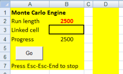
In Sheet 1, type the words from Figure 1 into A1, A2, A3, A4, and A7. In cell B2 you will enter
how many iterations you want. Cell B3 will be linked to a cell in this or another open
spreadsheet, and cell B4 will show you how far through the run you are. Column D will hold
all the Monte Carlo values generated.
Figure 1: Starting the Monte Carlo sheet
Cells A1 to B7 and column D have been colour coded to show the Monte Carlo area.
Now to write the macro named “MonteCarlo”. Click on the Developer tab and choose Macros.
Macro Name: MonteCarlo - Create. You will be taken to the Visual Basic Editor.
Type, or copy and paste these six lines between Sub MonteCarlo() and End Sub.
Range("D:D").ClearContents
n = Range("B2")
For q = 1 To n
Range("D1")(q) = Range("B3")
Range("B4") = q
Next
The macro clears column D at the start, reads how many Monte Carlo values you want from
B2, and then proceeds to copy the current value of cell B3 to the bottom of column D the
required number of times. After each transfer, it updates cell B4 with a progress report.
2
Spreadsheets in Education (eJSiE), Vol. 11, Iss. 1 [2018], Art. 1
https://epublications.bond.edu.au/ejsie/vol11/iss1/1
Find your way back to the spreadsheet itself either through View - Microsoft Excel, or by
pressing Alt+F11 or by clicking on the Excel icon at the far left of the menu ribbon.
Add a Form Control button. This is not essential but it looks smart and makes life easier.
Developer - Insert - Form Control - Button (top left) - outline where you want it to go with the
mouse just below A3. Assign Macro: MonteCarlo - OK. Right click on the button and edit the
text to “Go”. Later, when you click the button, the macro will run.
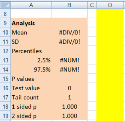
Type the words from Figure 2 into A9 to A19. Again, these have been colour coded to show
the Analysis section.
Figure 2: The remainder of the Monte Carlo sheet
Copy the other formulas. Some of these cells will show errors at this stage.
In cell type
B10 =AVERAGE(D:D)
B11 =STDEV(D:D)
B13 =PERCENTILE(D:D,A13)
B14 =PERCENTILE(D:D,A14)
B16 0
B17 =COUNT(D:D,B16)+1-MAX(RANK(B16,(D:D,B16),0),RANK(B16,(D:D,B16),1))
B18 =B17/COUNT(D:D,B16)
B19 =MIN(1,2*B18)
The reasons for the formulas in B16:B19 will be explained as they are needed.
Save As: Monte Carlo Master - Save as type: Excel Macro-Enabled Workbook - Save.
Your Monte Carlo Master spreadsheet is now ready to run although we will add to it later as
new functions become necessary. You can check it by typing 10 into cell B2 and =RAND() into
cell B3. Click Go. 10 random numbers should appear in column D.
Next time you open this spreadsheet you will probably be asked for permission to run the
macro. You can put the data you are working with either on the main Monte Carlo sheet we
have just made (Sheet 1) or on another worksheet in the Monte Carlo workbook. You can also
rename Sheet 1 as Monte Carlo by double clicking on the Sheet 1 tab at the bottom, and editing
the name to Monte Carlo. Having the working on the Monte Carlo sheet makes things slightly
3
Christie: Build your own Monte Carlo spreadsheet
Published by ePublications@bond, 2018
slower because of the time taken to continually update the screen, but it is interesting to see
the spreadsheet at work and it gives some appreciation of what is going on.
We will look at three examples of probability simulations, two methods of Monte Carlo
integration, four different randomization tests, and an example of Monte Carlo risk analysis.
These examples have all been part of student activities. Each example is best saved in its own
named workbook and closed before the next example is tried on the Monte Carlo Master sheet,
because the extra files working in the background slow the current sheet down.
3. Simulations
Excel has a limited range of randomization functions.
=RANDBETWEEN(low,high) will produce random whole numbers, uniformly distributed
between the given low and high numbers. This function is used in Examples 3.1 and 3.3
=RAND() will produce uniform random decimal numbers between 0 and 1. This can be
extended to a uniform distribution between two limits =low+(high-low)*RAND(). See
Examples 4.1 and 4.2.
RAND() can be used with the inverse normal function to generate random normal numbers
with any desired mean and SD. Use =NORMINV(RAND(),mean,SD). This is used in Example
3.2.
3.1. Simulation. Human randomizers
Statistics and psychology teachers sometimes do a class experiment to demonstrate how poor
a randomizer the human mind is. As homework, half the class is asked to toss a coin 200 times
and record the results in a grid. The other half is asked to fill out the grid with what they
imagine what 200 random coin tosses would look like. At the next class, the teacher can pick
out, almost at a glance and with a high degree of probability, the sheets of the human
randomizers. They are the ones which don’t have a run of six or more heads or tails. But just
how likely is it to get a run of at least six heads or six tails in a run of 200 coin tosses? This is a
very difficult problem to solve exactly. However, we can use the Monte Carlo sheet to make
an estimate.
On the main sheet at F1 type =RANDBETWEEN(0,1) and fill down to F200. (The
RANDBETWEEN(a,b) function selects a whole number from a to b so, for example,
=RANDBETWEEN(1,6) will simulate the roll of a die.) The 200 numbers in column F represent
200 coins with 1 being head and 0 being tail. In G6 type =SUM(F1:F6) and fill down to G200.
A 6 in column G means six heads in a row; a 0 means six tails in a row. In H6 type
=IF(OR(G6=0,G6=6),1,0) and fill down. This will give a 1 whenever column G shows a run of
six. In I6 type =IF(SUM(H:H)>0,1,0). This will be 1 whenever a run of at least six has occurred
somewhere in the 200 tosses. Press the F9 key to see a new run of 200.
In Run Length (cell B2) type, say, 2500. In Link cell (cell B3) type = I6 Enter, and click Go. After
2500 trials Mean (cell B10) holds the proportion of runs that have a run of six or more heads
or tails - a surprising approximately 97%. The rest of the numbers in the Analysis section are
irrelevant at this stage. Note that cell A7 tells you how to stop if some overenthusiastic person
puts in run length of 1000000.
4
Spreadsheets in Education (eJSiE), Vol. 11, Iss. 1 [2018], Art. 1
https://epublications.bond.edu.au/ejsie/vol11/iss1/1
Extension. Modify the sheet to estimate the probability of a run of 7 heads or tails (about 81%),
or a run of three sixes in 200 dice throws. (About 40%. See 3 Sixes in Supplementary Data).
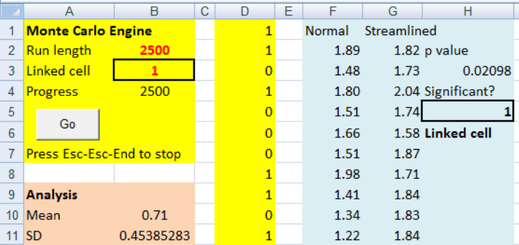
3.2. Simulation. Power and the paper helicopter
A favourite activity in some statistics classes is making paper helicopters. They provide a
simple way to get data for a designed experiment. See, for example the description at
http://www.paperhelicopterexperiment.com/. Each new class makes ten helicopters of both a
normal and a streamlined design. These are dropped from 2 m and the flight times are
recorded. The data is used as an introduction for the t test. Most years, the experiment results
in a significant difference being found, but not always. The data from various classes over
several years using the same design have averaged mean flight times of 1.55 s and 1.81 s for
the normal and streamlined versions respectively, and an overall SD of 0.22 s.
Set up a new Monte Carlo spreadsheet with the words in F1, G1, H2, and H4 from Figure 3.
Blue colour coding is used to show the Excel model of the problem.
Figure 3: The spreadsheet for the paper helicopters experiment
In this activity we need to generate random normal numbers. The general expression
=NORMINV(probability, mean, SD) returns the value which has the given proportion or
probability to its left. By making the probability a random number from 0 to 1, we get random
normal numbers with the desired mean and SD.
In cell F2 type =NORMINV(RAND(),1.55,0.22)
In cell G2 type =NORMINV(RAND(),1.81,0.22)
Copy these down to row 11 to simulate ten helicopters of each type.
In cell H3 type =TTEST(F2:F11,G2:G11,2,2). This gives the p value for the t test on those values.
The 2, 2 in the formula means a 2 tailed test assuming equal variances. The p value is the
probability that a difference at least as large as we observe could have happened by chance if,
in fact, there is no real difference between the groups. A common convention is that if the p
value is smaller than 0.05, then we are entitled to claim there is in fact a difference.
In cell H5 type =IF(H3<0.05,1,0). This will be 1 if p < 0.05, indicating a significant difference.
Fill in B2. Link B3 to H5 (type =H5 in cell B3). Click Go. B10 shows that the proportion of times
we get a significant result is about 70%. This is known as the power of this particular test
under these conditions.
5
Christie: Build your own Monte Carlo spreadsheet
Published by ePublications@bond, 2018
Extension. How many helicopters should we make in the future if we want to be 80% sure of
getting a significant result? The ranges in H3 will need to be expanded. (About 13 of each.)
Would it make a difference if we used 15 normal and 5 streamlined helicopters instead of 10
of each? (About 59% power which shows the benefit of a balanced design.)
3.3. Simulation. The birthday paradox
In a class of 30 students, what is the probability that at least two of them share a birthday?
This is an old problem made popular by Martin Gardner in his Scientific American column.
The probability can be calculated directly, but a Monte Carlo estimate can be quickly made.
In F1 type =RANDBETWEEN(1,365). This will give us a random day of the year. Fill down to
F30 for 30 students. In G1 type =COUNTIF(F:F,F1). This COUNTIF formula counts all the
occurrences in column F which match F1. Fill down. Most of column G will be 1 but if there is
a duplicate birthday, it will be 2 or more. In H1 type =IF(MAX(G:G)>1,1,0). This will give 1 if
there is a duplicate birthday, and 0 if there is not. Link this cell to B3 and Go. The Mean cell
B10, holds the probability of a duplicate birthday from 30 people- about 70%. The other
numbers in the analysis section can be ignored for this problem.
Extension. How many students for a 50% chance? (About 23.)
4. Monte Carlo integration
There are many situations where exact integration using calculus is very difficult, or even
impossible, and a numerical method must be used. In simple cases there are numerical
techniques like Simpson’s rule but as the number of variables increases, these methods
become too time and labour intensive. Demonstrations of two simple Monte Carlo integration
methods are illustrated in the next examples.
4.1. Monte Carlo hit or miss integration. Volume of a hypersphere
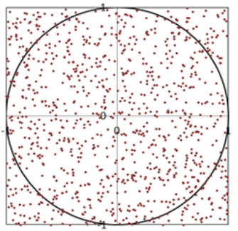
A common introduction to Monte Carlo integration is to find the area of a circle by scattering
a 2x2 square with random points. The area of the unit circle is estimated by multiplying the
area of the 2x2 square by the proportion of points lying within the circle. This process is
commonly known as “hit or miss” Monte Carlo integration. Figure 4 illustrates the idea.
Figure 4: Estimating the area of a circle
More interesting than this somewhat mundane activity, is estimating the volume of a unit 4
dimensional hypersphere by extending the same idea. We scatter a large number of random
6
Spreadsheets in Education (eJSiE), Vol. 11, Iss. 1 [2018], Art. 1
https://epublications.bond.edu.au/ejsie/vol11/iss1/1
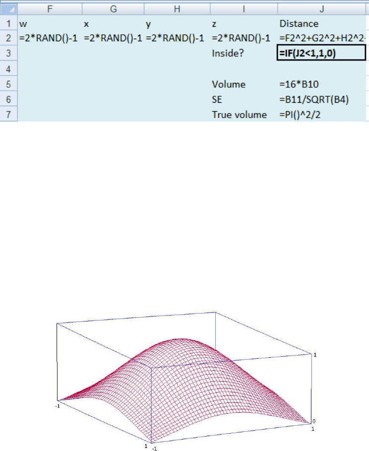
points inside a 2x2x2x2 hypercube, and find what proportion lie inside the hypercube. A point
(w, x, y, z) is inside the hypersphere if w² + x² + y² + z² < 1. The volume of a 2x2x2x2 hypercube
is 16, so our estimate of the volume of the hypersphere is the proportion of points inside the
hypersphere multiplied by 16. Use the formulas in Figure 5 and link B3 to J4. B10 will hold
the proportion of points inside the hypersphere.
Note that if you press Ctrl+~, Excel will show the formulas as in Figure 5. Ctrl+~ to return.
Figure 5: The formulas for the Monte Carlo hit or miss integration
The true value of the volume of a 4D hypersphere is given by V = π²/2. The uncertainty in
the estimate is given by the standard error = SD/n where n is the run length, so you can get
an idea of the accuracy of the estimate.
Extension. The sheet can be easily extended to yet higher dimensions. The unit circle, sphere
and 4D hypersphere have “volumes” of 3.142, 4.188 and 4.934 respectively. Is it true that the
volumes of hyperspheres will continue to increase as the dimension goes up? (Perhaps a little
surprisingly, the answer is no. See https://en.wikipedia.org/wiki/Volume_of_an_n-ball)
4.2. Sample mean Monte Carlo integration and the normal hump
Finding the volume under the surface
)(
22
yx
ez
+−
=
shown in Figure 6 for x and y between -1
and 1 is not an easy task, and impossible in most college calculus classes.
Figure 6: A “normal” hump
A Monte Carlo approach to finding this volume is to find the average height of the hump and
multiply by the base area; 2x2 = 4 in this case. Simply generate random x and y between -1
and 1 and collate the z values calculated. Average these z values and estimate the volume by
multiplying by the base area of 4. The true value is 2.231 to 3 decimal places. The accuracy of
the estimate is given by the standard error = SD/n.
7
Christie: Build your own Monte Carlo spreadsheet
Published by ePublications@bond, 2018
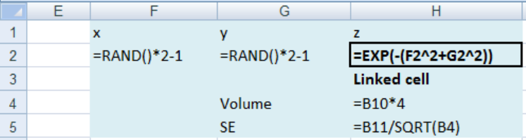
Figure 7: The volume of a normal hump by sample mean Monte Carlo integration
Extension. This problem can also be solved by the hit or miss method. Generate random points
(x, y, z) in the box. Include an IF to find the proportion of points below the surface. Multiply
by the volume of the box. How does the standard error of the hit or miss method compare
with that of the sample mean method for the same length run? (The hit or miss method is less
than half as accurate over the same run length in this case.)
5. Resampling, randomization and permutation tests
Much of classic statistics depends on the properties of the normal distribution. However,
Monte Carlo methods can be used in a much more natural way to solve the same problems
even if the data is not normal. Good (2005) [7] gives many examples that illustrate this aspect
of Monte Carlo analysis. Resampling assumes that the sample data you have is a good
representation of the population. It then effectively creates a virtual population using an
unlimited number of the same sample mixed together. When you take a new sample from this
virtual population, the same number can appear more than once. This is known a sampling
with replacement. This virtual population has the same mean, SD, and shape as our
representative sample. This can be accomplished with a new user defined function =pick(...).
The user defined function =perm() shuffles the data rows without replacement.
Open the Monte Carlo Master sheet. It is easy to get lost among all the Visual Basic screens.
An easy way to keep track is to go through the Developer - Macros - MonteCarlo - Edit and
add new material below the Monte Carlo macro. Copy these two user defined functions.
Function pick(Start)
Application.Volatile
w = Application.Caller.Columns.Count 'width of array
d = Application.Caller.Rows.Count 'depth of array
a = Start.Resize(d, w) 'puts original into a
b = a
For dd = 1 To d
r = Int(Rnd * d) + 1
For ww = 1 To w
b(dd, ww) = a(r, ww)
Next
Next
pick = b
End Function
Function perm(Start)
Application.Volatile
w = Application.Caller.Columns.Count 'width of array
d = Application.Caller.Rows.Count 'depth of array
a = Start.Resize(d, w) 'puts original into a
b = a
8
Spreadsheets in Education (eJSiE), Vol. 11, Iss. 1 [2018], Art. 1
https://epublications.bond.edu.au/ejsie/vol11/iss1/1

For dd = 1 To d
r = Int(Rnd * dd) + 1
For ww = 1 To w
b(dd, ww) = b(r, ww)
b(r, ww) = a(dd, ww)
Next
Next
perm = b
End Function
Return to the main Monte Carlo sheet (Alt+F11 or click the Excel icon) and save the Monte
Carlo Master workbook.
These two new functions are “array” functions. You highlight where you want the formula to
be, type the formula once and it is entered into the whole array of cells. Most importantly,
array functions are entered using Shift+Ctrl+Enter rather than the normal Enter.
Type 1 to 8 in F2:F9. Highlight G2:G9 and type =pick(F2). Hold down Shift+Ctrl and press
Enter. Now highlight H2:H9 and type =perm(F2). Shift+Ctrl+Enter. Press F9 for new sets.
Figure 8: The difference between =pick() and =perm()
5.1. Resampled confidence interval. Underwater video snapper survey
With normal data, there is an established method of finding a confidence interval for the
population mean from a sample using the standard error and the t distribution. When data is
not normal, the usual method will not work. Table 1 is the number of snapper seen in 22 baited
underwater video sites in a New Zealand marine reserve over one hour. A quick scan of the
data shows that the data is by no means normal. We want to find a 95% confidence interval
for the mean number of snapper per site.
Table 1: Number of snapper seen at 22 baited underwater video sites
1
0
10
12
11
2
0
0
12
4
15
0
6
1
0
9
0
25
0
2
1
9
Open a new Monte Carlo Master sheet. In column F put the 22 snapper numbers. This data is
also in the file Supplementary Data. In G3 type =AVERAGE(F2:F22). See Figure 9.
9
Christie: Build your own Monte Carlo spreadsheet
Published by ePublications@bond, 2018
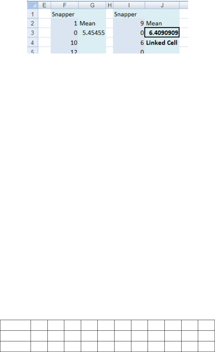
Figure 9: Setting up for a 95% confidence interval
Now make a second version of columns F and G in columns I and J. To do this, highlight
columns G and H by dragging over the column headings, hold down the Ctrl key, and drag
columns G and H across to I and J. At this stage the numbers in columns F and I will be
identical. We want to make a resampled version of F2:F22 in column I. This is where we can
use one of our new array functions where one formula fills up an entire array. Note that array
functions must be entered using the Ctrl, Shift, and Enter keys simultaneously.
Highlight the snapper numbers in I2:I22. Type =pick(F2) and press Ctrl-Shift-Enter.
Press the F9 key a few times to see what is happening. Note that the same snapper number
can occur more than once. Not every number must appear but every number has an equal
chance of occurring. This stage is now complete. The Monte Carlo average in J3 changes with
each new set of numbers.
Now for the Monte Carlo part. Put in the run length, say 2500. In the link cell B3 type =J3 Enter.
Now click Go. The 95% confidence interval for the population mean (B13:B14) is between
about 2.9 and 8.1 snapper per site. As a small teaching bonus, note that B11, the standard error,
has been calculated directly as being the standard deviation of all possible sample means, and
is effectively the same as the value given by using the usual formula SE = SD/n using the
original snapper data. The 95% confidence interval is not symmetric however, and so you
cannot calculate it from the SE alone, as you could with normal data.
5.2. A two sample resampling test. Bat calls
Project Echo was a bat monitoring program in Hamilton, NZ. Twenty seven bat detectors were
set up in various city locations - 11 in overgrown gullies and 16 in riverside walks. The number
of calls per detector over a single night is given in Table 2.
Is there evidence here that one environment has more calls than the other on average?
Table 2: Bat calls per night. Data also in Supplementary Data file.
Gully
3
2
1
3
0
2
0
50
8
2
1
River
73
7
1
18
0
0
10
0
25
0
44
1
0
53
1
1
A resampling test can be used when the data are not appropriate for a t test. Follow the general
idea of example 5.1. Put the two samples in columns F and G. In column H put suitable
formulas in H3, H5 and H7 for finding the difference in the means of the two samples. Copy
these three columns to the right and set up the sampling with replacement for each sample
separately using the =pick() array function as in example 5.1. Link B3 to the resampled
difference in L7, and put 0 in Test value in cell B16.
10
Spreadsheets in Education (eJSiE), Vol. 11, Iss. 1 [2018], Art. 1
https://epublications.bond.edu.au/ejsie/vol11/iss1/1
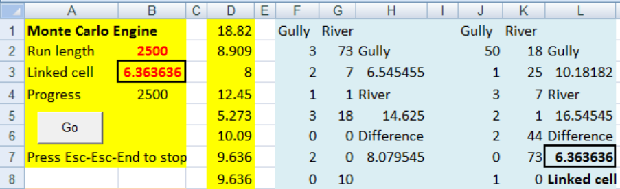
Figure 10: Bat calls. A two sample test
Cell B17, “Tail count” counts how many numbers in column D are as extreme as the “Test
value” in B16. After a suitable run, the significance or otherwise of the difference can be
established, either from the two sided p value or by inspecting the confidence interval for the
difference. Is the p value less than 0.05? No. It is about 0.3. Does the 95% confidence interval
include the value 0? Yes. 0 is inside the range -7 and 25 or thereabouts. No significant
difference has been shown between the habitats. It is worth noting that the 95% confidence
interval depends on the direction you define the difference. You may get -25 to 7, but the
conclusion is the same.
5.3. Permutation tests. Bat calls revisited
The permutation test is a different way of looking at the bat data. In example 5.2 using the
data in Table 2, we assumed that there could be a difference in the two areas and found a
confidence interval for that difference using resampling. A permutation test takes the more
sceptical position that there is no actual difference between the groups, and that any of the
values could have appeared in either of the groups. (In technical terms this is the “null
hypothesis”.) The test makes a list of all the differences that could potentially occur if that
were true by shuffling the data with no replacement at random through the groups. It then
compares the difference actually observed against the list of possible differences and finds
how likely it is to have happened by chance and calculates a p value.
Figure 11 shows how the data are put into a single list down to G28. This data is also in the
Supplementary Data file. In column H find the difference between the Means. Copy columns
F:H across to J:L. Highlight K2:K28 and type =perm(G2) Ctrl+Shift+Enter. Make the Test value
in B16 = H7. Link L7 to B3. Go.
11
Christie: Build your own Monte Carlo spreadsheet
Published by ePublications@bond, 2018
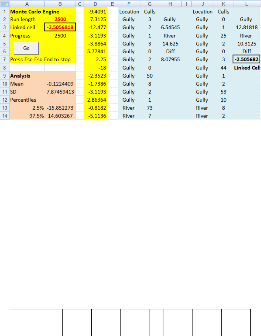
Figure 11: The sheet set up for a permutation test of the bat data.
The Monte Carlo sheet now makes a long list of potential differences and sees where the
observed difference of 8.08 fits in that list. The conclusion is the same as in Example 5.3. The
observed difference is not exceptional in the list of all possible differences.
5.4. Resampling with paired data. The FOG index
Many situations at the classroom level use paired data, particularly paired sample tests (use
=TTEST), correlation (use =CORREL), and regression (use =SLOPE).
As a more complex example using paired data we will find the confidence interval for the
reading level of a piece of text using the FOG index. The FOG reading index calculates the
appropriate reading level of a piece of text using the formula -
F = 0.4x(average words per sentence + % long words)
The result is the number of years of schooling needed to understand the text. (See
https://en.wikipedia.org/wiki/Gunning_fog_index or Gunning (1952) [8])
There is no formula for the standard error of the FOG index.
Table 3 gives the length of 13 sentences from a New Scientist article, along with the number
of “long” words in the sentence (words with more than two syllables). The data is paired so
we will need to keep that pairing.
Table 3: Sentence length and the number of long words in the sentence
Sentence No.
1
2
3
4
5
6
7
8
9
10
11
12
13
Length
33
4
21
19
16
45
14
32
23
15
4
10
33
Long Words
6
0
8
3
2
7
2
5
5
3
1
1
10
Columns F and G hold the paired data. This data is also in the Supplementary Data file. Put
in the appropriate Excel formulas.
H3 =AVERAGE(F2:F14)
H5 =SUM(G2:G14)/SUM(F2:F14)*100
H7 =0.4*(H3+H5)
See Figure 12. Copy columns F:H across to J:L using Ctrl and drag. Highlight both columns J2
to K14. Then type the array formula = pick(F2) and Ctrl+Shift+Enter. In B3 type = L7. Go.
12
Spreadsheets in Education (eJSiE), Vol. 11, Iss. 1 [2018], Art. 1
https://epublications.bond.edu.au/ejsie/vol11/iss1/1
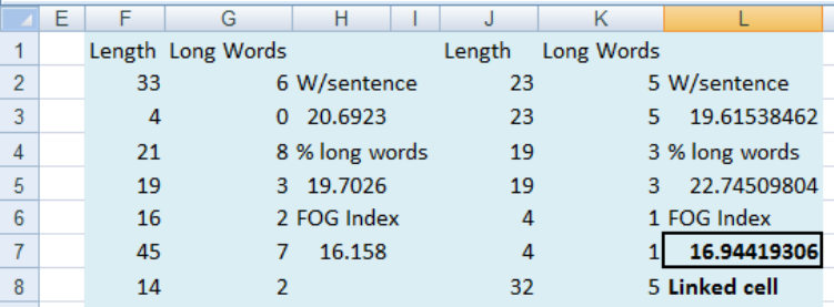
Figure 12: Resampling paired data
Note that it is possible for pairs to occur more than once, but the pairing is kept. The 95% CI
for the FOG index for this text is from about 13 to 19 years of education.
6. Monte Carlo risk analysis
Monte Carlo risk analysis is a method of determining the uncertainty in the answer of a
calculation where the inputs to that calculation are themselves uncertain. For each input, the
plausible distribution of values that could be taken by that input is determined either from
known data, a theoretical distribution, or from expert opinion. The calculation is then done
many times using a random selection of plausible inputs. The core ideas of Monte Carlo risk
analysis are -
• Every iteration should be a scenario which could occur in real life
• Every scenario which could occur in real life has a chance of being modelled
• The likelihood of any particular scenario arising in the analysis reflects the probability
of that scenario actually occurring in real life.
Every iteration of the calculation is a possible scenario which could be the true one. Later we
can analyse the large array of outputs to estimate the risk of getting any particular range of
values.
6.1. The Lucky Strike gold mine
You are the CEO of the Lucky Strike mine. If you know the number of tons of ore you can
extract a year, the number of grams of gold that can be extracted from each ton of ore, and the
price of gold, you can estimate the gross profit for the mine over the coming year. If at the
same time you know your overhead costs and how much it takes to extract and process each
ton of ore you can estimate the net annual profit for the mine.
Unfortunately, none of these numbers are known exactly for the coming year. Consequently,
the final answer from our calculation is only approximate and the true value remains
unknown. However, if we know or can estimate the range that the various numbers making
up the calculation can take, we can also estimate the range of possible values that the
calculated answer can have. A Monte Carlo risk analysis runs a large collection of potential
scenarios where the inputs are chosen at random from distributions which reflect the
likelihood of those inputs happening in real life.
13
Christie: Build your own Monte Carlo spreadsheet
Published by ePublications@bond, 2018
You meet with your management team, and assess the possible range of each input. Expert
opinion gives the values shown in Table 4. For example, your aim is to extract and process
one million tons of ore. 1,000,000 T is the most likely value but you may go a little over to
possibly 1,100,000 T. On the other hand unforeseen setbacks may mean that the mine may in
fact extract as little as 700,000 T at the very worst. The estimated profit using the most likely
value for each input is 19 million dollars, but what is the range of possible profits, and how
likely are we to reach the 19 million dollar goal? This data is also in the Supplementary Data
file.
Table 4: Input ranges for the Lucky Strike gold mine
Input
Minimum
Most likely
Maximum
Overheads $/year
900,000
1,000,000
1,200,000
Ore Extracted T/year
700,000
1,000,000
1,100,000
Mining Cost $/T ore
39
40
45
Processing Cost $/T ore
24
25
26
Ore Grade g/T gold
1.4
1.7
1.8
Gold price $/g gold
40
50
60
Earlier examples in this article have shown how to get random samples from uniform
distributions using the Excel functions =RAND() and =RANDBETWEEN(a,b), and from a
normal distribution using =NORMINV(RAND(),mean,SD). None of these distributions model
well the numbers in Table 4 which have a peak somewhere and fall off, some asymmetrically,
on each side. In many real life situations there is only a limited scope for improvement but
often a wide range of things that can go wrong. One simple and commonly used distribution
to model this sort of input is the triangular distribution. Few inputs in real life are exactly
triangular but we will use that distribution here as a convenient example. Unfortunately Excel
does not have a triangular function so we will write our own and save it in our Monte Carlo
spreadsheet for future use.
Developer - Macros - MonteCarlo - Edit and copy this code below the other functions.
Function tri(b, m, t)
Application.Volatile
If (t - b) * Rnd < m - b Then
tri = b + (m - b) * Rnd ^ 0.5
Else: tri = t - (t - m) * Rnd ^ 0.5
End If
End Function
Return to the spreadsheet (Alt F11). To use the new function type =tri(bottom, mode, top).
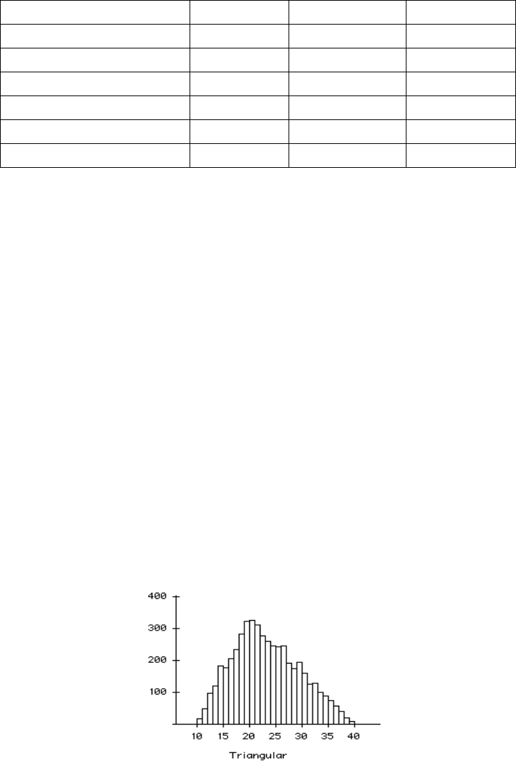
Figure 13 shows the result of 5000 numbers generated by =tri(10,20,40).
Figure 13: 5000 numbers from =tri(10,20,40)
14
Spreadsheets in Education (eJSiE), Vol. 11, Iss. 1 [2018], Art. 1
https://epublications.bond.edu.au/ejsie/vol11/iss1/1
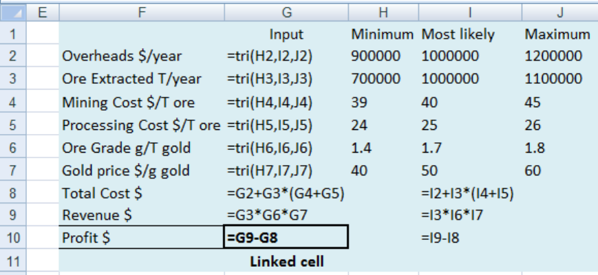
Back to Lucky Strike gold mine. On the Monte Carlo Master worksheet enter the data and
formulas shown in Figure 14.
Figure 14: Monte Carlo risk analysis for the Lucky Strike mine
Link the Profit to B3 as usual. When this is run a large number of feasible scenarios are
evaluated, and the output gives you the expected value and a 95% range of possible profits.
The expected profit is much less than the $19 million using just the most likely values.
Extensions. You can use the =PERCENTRANK(D:D,value) to find the likelihood of making a
profit less than the nominated value. The likelihood of making a loss is about 4% while the
likelihood of making more than $19 million is about 23%.
This scenario is loosely based on an idea from Chandoo.org.
7. Concluding remarks
Excel can generate random numbers from more distributions than those we have used so far.
The Bernoulli distribution. For example =IF(RAND()<0.7,1,0) will produce a sequence of 0s
and 1s, each of which has a 0.7 chance of being a 1 rather than a 0.
The Binomial distribution. For example =CRITBINOM(25,0.7,RAND()) will give a sequence of
numbers which could have been the number of successes from 25 trials if each trial has a 0.7
chance of success.
The Poisson distribution models the number of times a random event will occur if you know
how many you would have expected on average. Unfortunately there is no Excel function
which gives random Poisson variables directly. For small numbers up to about 40 you can use
the Binomial approximation to the Poisson. =CRITBINOM(100000,4.5/100000,RAND()) will
give a good approximation to a random Poisson variable of rate 4.5. The 100000 is the same in
every case. For rates above 40 the Normal approximation to the Poisson gives a reasonable
approximation. =INT(NORMINV(RAND(), 75,SQRT(75))) gives random Poisson variables
with average rate 75. The Monte Carlo Master given as supplementary material has a random
Poisson function already written. =Nrand(30) will produce random Poisson variables with
average rate 30. See also the Supplementary Materials for the appropriate code, and examples
of the function’s use.
15
Christie: Build your own Monte Carlo spreadsheet
Published by ePublications@bond, 2018
Once the basic ideas behind the spreadsheet have been understood, new applications can be
found in many different areas. See the Supplementary Material file for further ideas in each
of our four Monte Carlo topics.
8. References
[1] Albright, S. Christian, Winston, Wayne L. and Zappe, Christopher (1999). Data analysis
and decision making with Microsoft Excel. Duxbury Press.
[2] Christie, D. (2004), Resampling with Excel. Teaching Statistics, 26: 9–14
[3] Leong, Thin Yin Dr and Lee, Wee Leong Dr (2008) Spreadsheet data resampling for
Monte-Carlo simulation, Spreadsheets in Education (eJSiE): Vol. 3: Iss. 1, Article 6.
[4] Barr, Graham D. and Scott, Leanne D. (2013) Teaching statistical principles with a
roulette simulation, Spreadsheets in Education (eJSiE): Vol. 6: Iss. 2, Article 1.
[5] Rochowicz, John A. Jr (2010) Bootstrapping analysis, inferential statistics and Excel,
Spreadsheets in Education (eJSiE): Vol. 4: Iss. 3, Article 4.
[6] Botchkarev, Alexei (2015) Assessing Excel VBA suitability for Monte Carlo simulation,
Spreadsheets in Education (eJSiE): Vol. 8: Iss. 2, Article 3
[7] Good, P.I. (2005) Introduction to statistics through resampling methods and Microsoft Office
Excel. John Wiley & Sons
[8] Gunning, R. (1952) The technique of clear writing. McGraw-Hill, New York.
16
Spreadsheets in Education (eJSiE), Vol. 11, Iss. 1 [2018], Art. 1
https://epublications.bond.edu.au/ejsie/vol11/iss1/1
