Eco311 Optional Reading: Standard Error and Confidence Interval
(Jing Li, Miami University)
1. This note uses Monte Carlo simulation to help students understand concepts of stan-
dard error and confidence interval.
2. Statistics is about using samples to understand population. An important fact is that
there are many samples for a given population. For instance, the population can be
all students at Miami university. Then students taking a class in Laws Hall room
304 at 3pm on Monday can be a sample. Another sample can be students taking a
class in room FSB 0019, or students eating at Chipotle. Most likely, we get different
results from different samples. A key issue in statistics is accounting for the variation
or uncertainty in those different estimates.
3. Recall the math we did in class: if you obtain many random or iid samples, and
compute many sample means, then the variance of those many sample means is
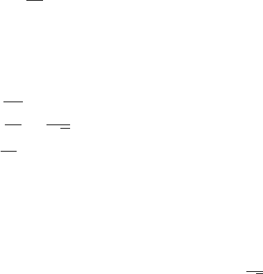
var(¯y) =
σ
2
n
(1)
where σ
2
= var(y) is the variance of data. The square root of var(¯y) is standard error
se, while the square root of var(y) is standard deviation sd:
se =
r
σ
2
n
=
σ
√
n
(2)
sd =
√
σ
2
= σ (3)
The former measures variation in ¯y, while the latter measures the variation in y. Do
not confuse them.
4. From (2) it is obvious that as the sample size n rises, the standard error
σ
√
n
falls.
This fact implies that as samples get larger, the variation in ¯y across different samples
gets smaller, or equivalently, ¯y becomes preciser. In light of this, the standard error
can serve as a measurement of uncertainty or unpreciseness of sample estimates. We
prefer precise estimates or small standard error. We can achieve that goal by using
large samples.
5. Next we run Monte Carlo simulation, and create a sample of 1000 observations of
1
random values that follow a Bernoulli distribution whose true population mean is
µ = P (y = 1) = 0.3.
The sample mean ¯y for this particular sample is 0.313, close to µ. The standard error
of ¯y is 0.01467127, and the 95 confidence interval for µ is (0.28421, 0.34179), which
contains the true value µ = 0.3.
> n = 1000
> library(purrr)
> set.seed(12345)
> ptrue = 0.3
> data = as.numeric(rbernoulli(n, p = ptrue))
> mean(data)
[1] 0.313
> se = sd(data)/sqrt(length(data))
> se
[1] 0.01467127
> t.test(data, conf.level = 0.95)$conf.int
[1] 0.28421 0.34179
6. To figure out the meaning of the standard error 0.01467127, let’s create another 10000
random samples (each has 1000 observations), and compute 10000 sample means
> iter = 10000
> v.ybar = rep(NA, iter)
> v.sd = rep(NA, iter)
> count95 = 0
> for (i in 1:iter) {
+ data = as.numeric(rbernoulli(n, p = ptrue))
+ n = length(data)
+ v.ybar[i]=mean(data)
+ v.sd[i] = sd(data)
+ count95 = count95 + (ptrue>v.ybar[i]-1.96*v.sd[i]/sqrt(n))*(ptrue<v.ybar[i]+1.96*v.sd[i]/sqrt(n))
+ }
> sd(v.ybar)
2
[1] 0.01463623
> count95/iter
[1] 0.9462
(a) The vector v.ybar stores the 10000 sample means. The first five sample means
are
> v.ybar[1:5]
[1] 0.323 0.300 0.283 0.289 0.294
It is clear that those five sample means vary. This illustrates sampling variation.
Because samples are large here, the five sample means are all close to µ = 0.3.
(b) The standard deviation of all 10000 sample means is
> sd(v.ybar)
[1] 0.01463623
which is very close to the standard error 0.01467127 we obtained before.
(c) Lesson 1: standard error measures the variation in the sample means.
(d) Next we compute the 95 confidence interval for each of the 10000 sample. The
lower and upper bounds are
v.ybar[i]-1.96*v.sd[i]/sqrt(n), v.ybar[i]+1.96*v.sd[i]/sqrt(n)
In the end we get 10000 confidence intervals. 94.62 percent or about 95 percent
of those intervals contain µ = 3.
(e) Lesson 2: if you were to take many random samples from the same population
and calculate a confidence interval from each sample, approximately 95 percent
of those intervals would contain the true population parameter. In other words,
you can be reasonably confident (95 percent confident) that the true parameter
lies within the given interval.
(f) Warning: it’s important to emphasize that the interpretation of confidence inter-
val does not mean that there is a 95 percent probability that the true parameter
lies within the interval; rather, it reflects the confidence in the estimation proce-
dure used to construct the interval.
3
