Query Optimization for Dynamic Graphs
Sutanay Choudhury
Pacific Northwest National
Laboratory, USA
sutanay[email protected]
Lawrence Holder
Washington State University,
USA
George Chin
Pacific Northwest National
Laboratory, USA
Patrick Mackey
Pacific Northwest National
Laboratory, USA
patrick.mac[email protected]v
Khushbu Agarwal
Pacific Northwest National
Laboratory, USA
khushbu.agarw[email protected]
John Feo
Pacific Northwest National
Laboratory, USA
john.f[email protected]
ABSTRACT
Given a query graph that represents a pattern of interest, the emerg-
ing pattern detection problem can be viewed as a continuous query
problem on a dynamic graph. We present an incremental algorithm
for continuous query processing on dynamic graphs. The algorithm
is based on the concept of query decomposition; we decompose a
query graph into smaller subgraphs and assemble the result of sub-
queries to find complete matches with the specified query. The nov-
elty of our work lies in using the subgraph distributional statistics
collected from the dynamic graph to generate the decomposition.
We introduce a “Lazy Search" algorithm where the search strategy
is decided on a vertex-to-vertex basis depending on the likelihood
of a match in the vertex neighborhood. We also propose a metric
named “Relative Selectivity" that is used to select between differ-
ent query decomposition strategies. Our experiments performed on
real online news, network traffic stream and a synthetic social net-
work benchmark demonstrate 10-100x speedups over competing
approaches.
1. INTRODUCTION
Social media streams and cyber data sources such as computer
network traffic are prominent examples of high throughput, dy-
namic graphs. Application domains such as computational jour-
nalism, emergency response, national security put a premium on
discovering critical events as soon as they emerge in the data. Thus,
processing streaming updates to a dynamic graph database for real-
time situational awareness is an important research problem. Apart
from their dynamic nature, these particular data sources are also
distinguished by their heterogeneous or multi-relational nature. For
example, a social media data stream contains a diverse set of en-
tity types such as person, movie, images etc. and relations such as
(friendship, like etc.). For cyber-security, a network traffic dataset
can be modeled as a graph where vertices represent IP addresses
and edges are typed by classes of network traffic [15]. Our work is
focused on continuous querying of these dynamic, multi-relational
graphs. We want to register a pattern as a graph query and con-
Permission to make digital or hard copies of all or part of this work for
personal or classroom use is granted without fee provided that copies are
not made or distributed for profit or commercial advantage and that copies
bear this notice and the full citation on the first page. To copy otherwise, to
republish, to post on servers or to redistribute to lists, requires prior specific
permission and/or a fee.
Copyright 20XX ACM X-XXXXX-XX-X/XX/XX ...$10.00.
tinuously perform the query on the data graph as it evolves over
time.
Continuous querying of a dynamic graph raises a number of
unique challenges. Indexing techniques that preprocess a graph
and speed up queries are expensive to periodically recompute in a
dynamic setting. Periodic execution of the query is an obvious so-
lution under this condition, but the effectiveness of this approach
will reduce as the interval between query executions shrinks. Also,
periodic searching of the entire graph can be wasteful where the
query match emerges slowly [6, 7] because we will find a partial
match for the query every time we search and potentially redo the
work numerous times.
The following describes the key idea behind our solution. We
approach the problem from an incremental processing perspective
where search happens locally on every edge arrival. We do not
search for the entire query graph around every new edge. Given
a query graph, we decompose it into smaller subgraphs as ordered
by their selectivity. The selectivity information is obtained using
the single-edge level and 2-edge path distribution obtained from
the graph stream (section 6). We store the resulting decomposition
into a data structure named SJ-Tree (Subgraph Join Tree) (section
3) that tracks matching subgraphs in the data graph. For a new edge
in the graph, we always search for the most selective subgraph of
the query graph. For other subgraphs of the query graph, a search
is triggered if and only if a match for the previous subgraph in the
selectivity order was obtained in the neighborhood of the new edge.
This algorithm named “Lazy Search" is described in section 5. We
introduce two metrics, Expected and Relative Selectivity, that cap-
tures the effectiveness of a given query decomposition (section 6).
Further, we demonstrate how these metrics can be used to reason
about the performance from different decompositions and select the
best performing strategy.
1.1 Contributions
The most important takeaway from our work is that even as the
subgraph isomorphism problem is NP-complete, it is possible to
perform efficient continuous queries on dynamic graphs by exploit-
ing the heterogeneity in the data and query graph. More specific
contributions from the paper are listed below.
1. We present a dynamic graph search algorithm that demon-
strates speedup of multiple orders of magnitude with respect
to the state of the art.
2. We introduce two selectivity metrics for query graphs that are
estimated using efficiently obtainable distributional statistics
of single edge and 2-edge subgraphs from the graph stream.
arXiv:1407.3745v1 [cs.DB] 14 Jul 2014
3. We present an automatic query decomposition algorithm that
selects the best performing strategy using the aforementioned
graph stream statistics and Relative Selectivity.
Our observations are supported by experiments on datasets from
three diverse domains (online news, computer network traffic and
a social media stream).
2. BACKGROUND AND RELATED WORK
This section is aimed at providing an overview of the related
field and provide the context for the studied problem. We begin
with introducing the key concepts.
Multi-Relational Graphs We define a graph G as an ordered-
pair G = (V, E) where V is the set of vertices and the E is
the set of edges that connect the vertices. An edge represents a
pair of vertices, also known as end points. In the following, we
use V (G) and E(G) to indicate the set of vertices and edges as-
sociated with a graph G. A labeled graph is a six-tuple G =
(V, E, Σ
V
, Σ
E
, λ
V
, λ
E
), where Σ
V
and Σ
E
are sets of distinct
labels for vertices and edges. λ
V
and λ
E
are vertex and edge la-
beling functions, i.e. λ
V
: V → Σ
V
and λ
E
: E → Σ
E
.
Dynamic Graphs We define dynamic graphs as graphs that are
changing over time through edge insertion or deletion. Every edge
in a dynamic graph has a timestamp associated with it and there-
fore, for any subgraph g of a dynamic graph we can define a time
interval τ(g) which is equal to the interval between the earliest and
latest edge belonging to g. We focus on directed, labeled dynamic
graphs with multi-edges in this work. The graph is maintained as
a window in time. Given a time window t
W
, edges are deleted as
they become older than t
last
− t
W
, where t
last
is the timestamp of
the newest edge in the graph.
Continuous Queries A continuous query can be described as
computing a function f over a stream S continuously over time
and notifying the user whenever the output of f satisfies a user-
defined constraint [18]. They are distinguished from ad-hoc query
processing by their high selectivity (looking for unique events) and
need to detect newer updates of interest as opposed to retrieving
lots of past information. In this paradigm the primary objective
is to notify a listener as soon as the query is matched. One may
view conventional databases as passive repositories with large col-
lections of data that work in a request-response model whereas con-
tinuous queries are data-driven or trigger oriented. These features
challenge many of the fundamental assumptions for conventional
databases and establish continuous query processing on relational
data streams as a major research area. The literature on database
research from the past two decades is abundant with work on con-
tinuous query systems [1,4]. Babcock et al. [2] provide an excellent
overview of continuous query systems and their design challenges.
Subgraph Isomorphism Given the query graph G
q
and a match-
ing subgraph of the data graph (G
d
) denoted as G
0
d
, a matching be-
tween G
q
and G
0
d
involves finding a bijective function f : V (G
q
) →
V (G
0
d
) such that for any two vertices u
1
, u
2
∈ V (G
q
), (u
1
, u
2
) ∈
E(G
q
) ⇒ (f(u
1
), f(u
2
)) ∈ E(G
0
d
).
2.1 Problem Statement
Every edge in a dynamic graph has a timestamp associated with
it and therefore, for any subgraph g of a dynamic graph we can de-
fine a time duration τ (g) which is equal to the duration between
the earliest and latest edge belonging to g. Given a dynamic multi-
relational graph G
d
, a query graph G
q
and a time window t
W
, we
report whenever a subgraph g
d
that is isomorphic to G
q
appears
in G
d
such that τ(g
d
) < t
W
. The isomorphic subgraphs are also
referred to as matches in the subsequent discussions. Assume that
G
k
d
is the data graph at time step k. If M(G
k
d
) is the cumulative
set of all matches discovered until time step k and E
k+1
is the set
of edges that arrive at time step k + 1, we present an algorithm to
compute a function f (G
d
, G
q
, E
k+1
) which returns the incremen-
tal set of matches that result from updating G
d
with E
k+1
and is
equal to M(G
k+1
d
) − M(G
k
d
).
2.2 Related Work
Graph querying techniques have been studied extensively in the
field of pattern recognition over nearly four decades [8]. Two pop-
ular subgraph isomorphism algorithms were developed by Ullman
[24] and Cordella et al. [9]. The VF2 algorithm [9] employs a filter-
ing and verification strategy and outperforms the original algorithm
by Ullman. Over the past decade, the database community has
focused strongly on developing indexing and query optimization
techniques to speed up the searching process. A common theme
of such approaches is to index vertices based on k-hop neighbor-
hood signatures derived from labels and other properties such as
degrees and centrality [22, 23, 27]. Other major areas of work in-
volve exploration of subgraph equivalence classes [11] and search
techniques for alternative representations such as similarity search
in a multi-dimensional vector space [16]. Apart from neighborhood
based signatures, graph sketches is an important area that focuses
on generating different synopses of a graph data set [26]. Develop-
ment of efficient graph sketching algorithms and their applications
into query estimation is expected to gain prominence in the near
future.
Investigation of subgraph isomorphism for dynamic graphs did
not receive much attention until recently. It introduces new algo-
rithmic challenges because we can not afford to index a dynamic
graph frequently enough for applications with real-time constraints.
In fact this is a problem with searches on large static graphs as
well [21]. There are two alternatives in that direction. We can
search for a pattern repeatedly or we can adopt an incremental ap-
proach. The work by Fan et al. [10] presents incremental algo-
rithms for graph pattern matching. However, their solution to sub-
graph isomorphism is based on the repeated search strategy. Chen
et al. [5] proposed a feature structure called the node-neighbor tree
to search multiple graph streams using a vector space approach.
They relax the exact match requirement and require significant pre-
processing on the graph stream. Our work is distinguished by its
focus on temporal queries and handling of partial matches as they
are tracked over time using a novel data structure. From a data-
organization perspective, the SJ-Tree approach has similarities with
the Closure-Tree [12]. However, the closure-tree approach assumes
a database of independent graphs and the underlying data is not dy-
namic. There are strong parallels between our algorithm and the
very recent work by Sun et al. [21], where they implement a query-
decomposition based algorithm for searching a large static graph
in a distributed environment. Here our work is distinguished by
the focus on continuous queries that involves maintenance of par-
tial matches as driven by the query decomposition structure, and
optimizations for real-time query processing. Mondal and Desh-
pande [19] propose solutions to supporting continuous ego-centric
queries in a dynamic graph, Our work focuses on subgraph isomor-
phism, while [19] is primarily focused on aggregate queries. We
view this as complementary to our work, and it affirms our belief
that continuous queries on graphs is an important problem area,
and new algorithms and data structures are required for its devel-
opment.
3. A QUERY DECOMPOSITION APPROACH
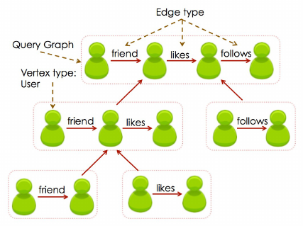
Figure 1: Illustration of the decomposition of a social query in
SJ-Tree.
We introduce an approach that guides the search process to look
for specific subgraphs of the query graph and follow specific tran-
sitions from small to larger matches. Following are the main intu-
itions that drive this approach.
1. Instead of looking for a match with the entire graph or just
any edge of the query graph, partition the query graph into
smaller subgraphs and search for them.
2. Track the matches with individual subgraphs and combine
them to produce progressively larger matches.
3. Define a join order in which the individual matching sub-
graphs will be combined. Do not look for every possible
way to combine the matching subgraphs.
Figure 1 shows an illustration of the idea. Although the current
work is completely focused on temporal queries, the graph decom-
position approach is suited for a broader class of applications and
queries. The key aspect here is to search for substructures with-
out incurring too much cost. Even if some subgraphs of the query
graph are matched in the data, we will not attempt to assemble the
matches together without following the join order.
The query decomposition approach can still suffer from having
to maintain too many partial matches. If a subgraph of the query
graph is highly frequent, we will end up tracking a large number
of partial matches corresponding to that subgraph. Unless we have
quantitative knowledge about how these partial matches transition
into larger matches, we face the risk of tracking a large number of
non-promising matching subgraphs. The “Lazy Search" approach
outlined earlier in the introduction enhances this further. For any
new edge, we search for a query subgraph if and only if it is the
most selective subgraph in the query or if one of the either ver-
tices in that edge participates in a match with the preceding (query)
subgraph in the join order.
This section is dedicated towards introducing the data structures
and algorithms for dynamic graph search. We begin with introduc-
ing the SJ-Tree structure (section 3.1) and then proceed to present
the basic algorithms (Algorithm 1 and 2). The “Lazy Search"-
enhanced version is introduced later in section 5. Automated gen-
eration of SJ-Tree is covered in section 6.
3.1 Subgraph Join Tree (SJ-Tree)
We introduce a tree structure called Subgraph Join Tree (SJ-
Tree). SJ-Tree defines the decomposition of the query graph into
smaller subgraphs and is responsible for storing the partial matches
to the query. Figure 1 shows the decomposition of an example
query. Each of the rectangular boxes with dotted lines will be rep-
resented as a node in the SJ-Tree. The query subgraphs shown in-
side each “box" will be stored as a node property described below.
DEFINITION 3.1.1 A SJ-Tree T is defined as a binary tree com-
prised of the node set N
T
. Each n ∈ N
T
corresponds to a subgraph
of the query graph G
q
. Let’s assume V
SG
is the set of correspond-
ing subgraphs and |V
SG
| = |N
T
|. Additional properties of the
SJ-Tree are defined below.
DEFINITION 3.1.2 A Match or a Partial Match is as a set of
edge pairs. Each edge pair represents a mapping between an edge
in a query graph and its corresponding edge in the data graph.
DEFINITION 3.1.3 Given two graphs G
1
= (V
1
, E
1
) and G
2
=
(V
2
, E
2
), the join operation is defined as G
3
= G
1
1 G
2
, such
that G
3
= (V
3
, E
3
) where V
3
= V
1
∪ V
2
and E
3
= E
1
∪ E
2
.
PROPERTY 1. The subgraph corresponding to the root of the SJ-
Tree is isomorphic to the query graph. Thus, for n
r
= root{T },
V
SG
{n
r
} ≡ G
q
.
PROPERTY 2. The subgraph corresponding to any internal node
of T is isomorphic to the output of the join operation between the
subgraphs corresponding to its children. If n
l
and n
r
are the left
and right child of n, then V
SG
{n} = V
SG
{n
l
} 1 V
SG
{n
r
}.
Therefore, each leaf of the SJ-Tree represent subgraphs that we
want to search for (perform subgraph isomorphism) on the stream-
ing updates. Internal nodes in the SJ-Tree represents subgraphs
that result from the joining of subgraphs returned by the subgraph
isomorphism operations.
PROPERTY 3. Each node in the SJ-Tree maintains a set of matches.
We define a function matches(n) that for any node n ∈ N
T
, re-
turns a set of subgraphs of the data graph. If M = matches(n),
then ∀G
m
∈ M, G
m
≡ V
SG
{n}.
PROPERTY 4. Each internal node n in the SJ-Tree maintains a
subgraph, CUT-SUBGRAPH(n) that equals the intersection of the
query subgraphs of its child nodes.
For any internal node n ∈ N
T
such that CUT-SUBGRAPH(n) 6=
∅, we also define a projection operator Π. Assume that G
1
and G
2
are isomorphic, G
1
≡ G
2
. Also define Φ
V
and Φ
E
as functions
that define the bijective mapping between the vertices and edges of
G
1
and G
2
. Consider g
1
, a subgraph of G
1
: g
1
⊆ G
1
. Then g
2
=
Π(G
2
, g
1
) is a subgraph of G
2
such that V (g
2
) = Φ
V
(V (g
1
))
and E(g
2
) = Φ
E
(E (g
1
)).
Our decision to use a binary tree as opposed to an n-ary tree is
influenced by the simplicity and lowering the combinatorial cost
of joining matches from multiple children. With the properties of
the SJ-Tree defined, we are now ready to describe the graph search
algorithm.
3.2 Dynamic Graph Search Algorithm
We begin with describing our dynamic graph search algorithm
(Algorithm 1 and 2). The input to DYNAMIC-GRAPH-SEARCH
is the dynamic graph so far G
d
, the SJ-Tree (T ) corresponding to
the query graph and the set of incoming edges. Every incoming
edge is first added to the graph (Algorithm 1, line 3). Next, we
iterate over all the query subgraphs to search for matches contain-
ing the new edge (line 5-6). Any discovered match is added to the
SJ-Tree (line 9).
Next, we describe the UPDATE-SJ-TREE function. Each node

Algorithm 1 DYNAMIC-GRAPH-SEARCH(G
d
, T, edges)
1: leaf-nodes =GET-LEAF-NODES(T )
2: for all e
s
∈ edges do
3: UPDATE-GRAPH(G
d
, e
s
)
4: for all n ∈ leaf-nodes do
5: g
q
sub
=GET-QUERY-SUBGRAPH(T, n)
6: matches =SUBGRAPH-ISO(G
d
, g
q
sub
, e
s
)
7: if matches 6= ∅ then
8: for all m ∈ matches do
9: UPDATE-SJ-TREE(T, n, m)
in the SJ-Tree maintains its sibling and parent node information
(Algorithm 2, line 1-2). Also, each node in the SJ-Tree maintains
a hash table (referred by the match-tables property in Algorithm 2,
line 4). GET() and ADD() provides lookup and update operations
on the hash tables. Each entry in the hash table refers to a Match.
Whenever a new matching subgraph g is added to a node in the SJ-
Tree, we compute a key using its projection (Π(g)) and insert the
key and the matching subgraph into the corresponding hash table
(line 12). When a new match is inserted into a leaf node we check
to see if it can be combined (referred as JOIN()) with any matches
that are contained in the collection maintained at its sibling node.
A successful combination of matching subgraphs between the leaf
and its sibling node leads to the insertion of a larger match at the
parent node. This process is repeated recursively (line 11) as long
as larger matching subgraphs can be produced by moving up in the
SJ-Tree. A complete match is found when two matches belonging
to the children of the root node are combined successfully.
EXAMPLE Let us revisit Figure 1 for an example. Assuming we
find a match with the query subgraph containing a single “friend"
edge (e.g. {(“George", “friend", “Sutanay")}), we will probe the
hash table in the leaf node with “likes" edges. If the hash table
stored a subgraph such as {(“Sutanay", “likes", “Santana")}, the
JOIN() will produce a 2-edge subgraph {(“George", “friend", “Su-
tanay"), (“Sutanay", “likes", “Santana")}. Next, it will be inserted
into the parent node with 2-edges. The same process will be sub-
sequently repeated, beginning with the probing of the hash table
storing matches with subgraphs with a “follows" edge.
Algorithm 2 UPDATE-SJ-TREE(node, m)
1: sibling = sibling[node]
2: parent = parent[node]
3: k =GET-JOIN-KEY(CUT-SUBGRAPH[parent], m)
4: H
s
= match-tables[sibling]
5: M
k
s
= GET(H
s
, k)
6: for all m
s
∈ M
k
s
do
7: m
sup
= JOIN(m
s
, m)
8: if parent = root then
9: PRINT(’MATCH FOUND : ’, m
sup
)
10: else
11: UPDATE-SJ-TREE(parent, m
sup
)
12: ADD(match-tables[node], k, m)
4. ANALYSIS OF DYNAMIC GRAPH SEARCH
ALGORITHM
At this point, it is probably obvious that different SJ-Tree struc-
tures can be generated from the same query graph. Later in the pa-
per, we provide example query decompositions in Figure 8. While
multiple factors can lead to generation of different SJ-Trees, one
primary factor is our choice for granularity of decomposition, the
size and the structure of the subgraphs we decompose the query
to. As we will establish through extensive analysis through this
paper, there is value in establishing a standard set of small sub-
graphs that are efficient to search for in a real-time setting. Hence-
forth, we often refer to these set of small subgraphs as search prim-
itives or simply primitives. As a first step to understand the speed-
memory tradeoff associated with different choices for primitives,
we begin with the complexity analysis of the dynamic graph search
described in Algorithm 1 and 2. A key operation in Algorithm 1 is
the process of subgraph isomorphism around every new edge in the
graph. Therefore, we exclusively focus on the complexity analysis
in terms of 1-3 edge subgraphs as candidates for search primitives.
SINGLE EDGE SUBGRAPHS When the query graph (g
q
sub
in Al-
gorithm 1, line 5) contains a single edge, checking if an edge from
the data graph (e
s
) matches the query edge require comparing the
types and potentially other attributes of the edges. Depending on
the query constraint, we may need to look up the node label to
perform a string comparison or evaluate a regular expression. The
node labels or any other node-specific properties are stored in an
array leading to constant time access to node labels. Therefore, a
single-edge query can be matched in O(1) time.
TRIADS Assume that the query graph is a triad with three ver-
tices v
1
, v
2
and v
3
, and edges ordered as e
1
= (v
1
, v
2
), e
2
=
(v
2
, v
3
), e
3
= (v
3
, v
1
). For any edge e in the data graph, we can
detect a match with e
1
in constant time. If e is matched, we search
the neighborhood of the vertex that matches with v
2
to search for
e
2
. Denoting this vertex as v
0
2
, the cost of this second level of search
is O(degree(v
0
2
)). In case of a 3-edge subgraph, each of the suc-
cessful second level searches proceed to find a match for the third
edge. Thus, the cost of a 2-edge subgraph is O(degree(v
0
2
)) and
a 3-edge subgraph is O(degree(v
0
2
) ∗ degree(v
0
3
)). We can refine
these estimates to obtain an average cost of the search as O(
¯
d
2
) for
a 2-edge subgraph and O(
¯
d
2
¯
d
3
) for a 3-edge subgraph, where
¯
d
2
and
¯
d
3
are the average degree of the vertices in the graph for the
types of v
2
and v
3
.
The next step is to estimate a cost for the SJ-Tree update opera-
tion (Algorithm 2). We begin with the hash-join operation (Algo-
rithm 2, line 7).
Assume the frequency of a graph g
i
q
is n
i
, where the frequency
of a subgraph is defined as the count of its instances over an edge
stream of length N. Therefore, over N edges, we can expect O(n
1
)
matches for g
1
q
and O(n
2
) matches for g
2
q
. Therefore, H
2
(hash
table associated with the SJ-Tree node representing g
2
q
) will be
probed for a match O(n
1
) times over N edges and H
1
(associ-
ated with the SJ-Tree node representing g
1
q
) will be probed O(n
2
)
times within the same period.
If we knew the frequency of G
q
, henceforth referred as f
S
(G
q
),
then we can also estimate the number of new subgraphs that will be
produced as the result of the hash-joins. Given that the frequency of
the larger subgraph can not exceed that of the more selective com-
ponent we can approximate O(n(G
q
)) ' min (O(n
1
), O(n
2
))).
Therefore, the average work for every incoming edge in the graph
can be expressed as,
f
S
(g
1
q
) + f
S
(g
2
q
) + O(n
1
) + O(n
2
) + min (O(n
1
), O(n
2
)))
/N.
The Hash-Join combined with leaf level searches provides the
simplest example of a SJ-Tree, a binary tree with height 1. In this
section, we analyze the time complexity of the query processing as
it happens in a multi-level SJ-Tree. Given any non-leaf node n, we
can obtain the expression for average work by adapting the com-
plexity expression shown above. Note that if a child of n, denoted
by n
c
, is not a leaf level node but an internal node, then the term

corresponding to the search cost (f
S
(g)) disappears. Additionally,
we can replace the search cost with the cost corresponding to the
average work incurred by the subtree rooted by n
c
. Therefore,
given a SJ-Tree (T
sj
) the average work (C(T
sj
)) can be obtained
by recursive computation from the root. C(T
sj
) = C(root(T
SJ
))
5. LAZY SEARCH
Revisiting our example from Figure 1, it is reasonable to assume
that the “friend" relation is highly frequent in the data. If we de-
composed the query graph all the way to single edges then we will
be tracking all edges that match “friend". Clearly, this is waste-
ful. One may suggest decomposing the query to larger subgraphs.
However, it will also increase the average time incurred in per-
forming subgraph isomorphism. Deciding the right granularity of
decomposition requires significant knowledge about the dynamic
graph. This motivates us to introduce a new algorithmic extension.
Assume the query graph G
q
is partitioned into two subgraphs
g
1
and G
1
q
. We use the notation G
k
q
to indicate what remains of
G
q
after the k-th iteration in the decomposition process. If the
probability of finding a match for g
1
is less than the probability
of finding a match for G
1
q
, then it is always desirable to search
for g
1
and look for G
1
q
only where an occurrence of g
1
is found.
Therefore, we select g
1
to be the most selective edge or 2-edge
subgraph in the query graph and always search for g
1
around every
new edge in the graph. Once we detect subgraphs in G
d
that match
with g
1
, we follow the same approach to search for G
q
in their
neighborhood. We partition G
1
q
further into two subgraphs: g
2
and
G
2
q
, where g
2
is another 1-edge or 2-edge subgraph.
DATA STRUCTURES With the SJ-Tree, the partitioning of G
q
is
done upfront at the query compile time with g
1
, g
2
etc becoming
the leaves of the tree. The main difference between Lazy Search
and that of Algorithm 2 is that we will be searching for g
2
only
around the edges in G
d
where a match with g
1
is found. Therefore,
for every vertex u in G
d
, we need to keep track of the g
i
-s such
that u is present in the matching subgraph for g
i
. We use a bitmap
structure M
b
to maintain this information. Each row in the bitmap
refers to a vertex in G
d
and the i-th column refers to g
i
, or the i-
th leaf in the SJ-Tree. If the search for subgraph g
i
is enabled for
vertex u in G
d
, then M
b
[u][i] = 1 and zero otherwise. Whenever
a matching subgraph g
0
for g
i
is discovered, we turn on the search
for g
i+1
for all vertices in V (g
0
). This is accomplished by setting
M
b
[v][i + 1] = 1 where v ∈ V (g
0
).
ROBUSTNESS WITH SUBGRAPH ARRIVAL ORDER Consider a
SJ-Tree with just two leaves representing query subgraphs g
1
and
g
2
, with g
1
representing the more selective left leaf. The above
strategy is not robust to the arrival order of matches. Assume g
0
1
and g
0
2
are subgraphs of G
d
that are isomorphic to g
1
and g
2
re-
spectively. Together, g
0
1
× g
0
2
is isomorphic to the query graph G
q
.
Because we are searching for g
1
on every incoming edge, g
0
1
will
be detected as soon as it appears in the data graph. However, we
will detect g
0
2
only if appears in G
d
after g
0
1
. If g
0
2
appeared in G
d
before g
0
1
we will not find it because we are not searching for g
2
all
the time.
We introduce a small change to address this temporal ordering
issue. Whenever we enable the search on a node in the data graph,
we also perform a subgraph search around the node to find any
match that has occurred earlier. Thus, when we find g
1
and enable
the search for g
2
on every subsequent edge arrival, we also perform
a search in G
d
looking for g
1
. This ensures that we will find g
2
even if it appeared before g
1
.
Algorithm 3 summarizes the entire process. Lines 2-3 loop over
all news edges arriving in the graph and update the graph. Next,
given a new edge e
s
, for each node in the SJ-Tree, we check to see
if we should be searching for its corresponding subgraph around
e
s
(lines 4-8). The DISABLED() function queries the bitmap in-
dex and returns true if the corresponding search task is disabled.
GET-QUERY-SUBGRAPH returns the query subgraph g
q
sub
corre-
sponding to node n in the SJ-Tree (line 9). Next, we search for
g
q
sub
using a subgraph-isomorphism routine that only searches for
matches containing at least one of the end-point vertices of e
s
(u
and v, mentioned in line 5-6). For each matching subgraph found
containing u or v, we enable the search for the query subgraph
corresponding the sibling of n in the SJ-Tree. If n was not left-
deep most node in the SJ-Tree, then we also query the left sibling
to probe for potential join candidates (QUERY-SIBLING-JOIN(),
line 16). Any resultant joins are pushed into the parent node and
the entire process is recursively repeated at one level higher in the
SJ-Tree.
Algorithm 3 LAZY-SEARCH(G
d
, T, edges)
1: leaf-nodes =GET-LEAF-NODES(T )
2: for all e
s
∈ edges do
3: UPDATE-GRAPH(G
d
, e
s
)
4: for all n ∈ leaf-nodes do
5: u =src(e
s
)
6: v =dst(e
s
)
7: if DISABLED(u, n) AND DISABLED(v, n) then
8: continue
9: g
q
sub
=GET-QUERY-SUBGRAPH(T, n)
10: matches =SUBGRAPH-ISO(G
d
, g
q
sub
, e)
11: for all m ∈ matches do
12: if n = 0 then
13: ENABLE-SEARCH-SIBLING(n, m)
14: else
15: M
j
= QUERY-SIBLING-JOIN(n, m)
16: p = PARENT(n)
17: for all m
j
∈ M
j
do
18: UPDATE(p, m
j
)
19: ENABLE-SEARCH-SIBLING(p, m)
6. SJ-TREE GENERATION
Here we address the topic of automatic generation of the SJ-Tree
from a specified query graph. We begin with introducing key defi-
nitions, followed by the decomposition algorithm.
DEFINITION Subgraph Selectivity Given a large typed, directed
graph G, the selectivity of a typed, directed subgraph g with k-
edges (denoted as S(g)) is the ratio of the number of occurrences
of g and the total number of all k-edge subgraphs in G. Instances
of g may overlap with each other.
DEFINITION Selectivity Distribution The selectivity distribu-
tion of a set of subgraphs G
k
is a vector containing the selectiv-
ity for every subgraph in G
k
. The subgraphs are ordered by their
frequencies in ascending order.
We present a greedy algorithm (Algorithm 4) for decomposing
a query graph into its subgraphs and generating a SJ-Tree. Our
choice for the greedy heuristic is motivated by extensive survey
of the literature on optimal join order determination in relational
databases [13, 17, 25]. A key conclusion of the survey states that
left-deep join plans (or left deep binary trees in this case) is one
of the best performing heuristics. The above mentioned studies
point to a large body of research using techniques such as dynamic
programming and genetic algorithms to find the optimal join or-
der. Nonetheless, finding the lowest cost join order or using a cost-

driven join order determination remains an interesting problem in
graph databases, and the approaches based on minimum spanning
trees or approximate vertex cover can provide an initial path for-
ward.
Inputs to Algorithm 4 are the query graph G
q
and an ordered set
of primitives M. Our goal is to decompose G
q
into a collection
of (possibly repeated) subgraphs chosen from M . Entries of M
are sorted in ascending order of their subgraph selectivity. Given
a query graph G
q
, the algorithm begins with finding the subgraph
with the lowest selectivity in M. This subgraph is next removed
from the query graph and the nodes of the removed subgraph are
pushed into a “frontier" set. We proceed by searching for the next
selective subgraph that includes at least one node from the fron-
tier set. We continue this process until the query graph is empty.
SUBGRAPH-ISO performs a subgraph isomorphism operation to
find an instance of g
M
in G
q
. Algorithm 4 uses two versions of
SUBGRAPH-ISO. The first version uses three arguments, where
the second argument is a vertex id v. This version of SUBGRAPH-
ISO searches G
q
for instances of g
M
by only searching in the
neighborhood of v. The other version accepting two arguments
searches entire G
q
for an instance of g
M
. REMOVE-SUBGRAPH
accepts two graphs as argument, where the second argument (g
sub
)
is a subgraph of the first graph (G
q
). It removes all edges in G
q
that belong to g
sub
. A vertex is removed from G
q
only when the
edge removal results in a disconnected vertex.
Algorithm 4 BUILD-SJ-TREE(G
q
, M)
1: frontier = ∅
2: while |V (G
q
)| > 0 do
3: g
sub
= ∅
4: for all g
M
∈ M do
5: if frontier 6= ∅ then
6: for all v ∈ frontier do
7: g
sub
=SUBGRAPH-ISO(G
q
, v, g
M
)
8: break
9: else
10: g
sub
=SUBGRAPH-ISO(G
q
, g
M
)
11: if g
sub
6= ∅ then
12: frontier = f rontier ∪ V (g
sub
)
13: G
q
=REMOVE-SUBGRAPH(G
q
, g
sub
)
6.1 Selectivity Estimation of Primitives
We propose computing the selectivity distribution of primitives
by processing an initial set of edges from the graph stream. For
experimentation purposes we assume that the selectivity order re-
mains the same for the dynamic graph when we perform the query
processing. This work does not focus on modeling the accuracy of
this estimation. Modeling the impact on performance when the ac-
tual selectivity order deviates from the estimated selectivity order
is an area of ongoing work.
Which subgraphs are good candidates as entries of M? Fol-
lowing are two desirable properties for entries in M : 1) the cost
for subgraph isomorphism should be low. 2) Selectivity estimation
of these subgraphs should be efficient as we will need to periodi-
cally recompute the estimates from a graph stream. Based on these
two criteria, we select single edge subgraphs and 2-edge paths as
primitives in this study. Computing the selectivity distribution for
single-edge subgraphs resolves to computing a histogram of vari-
ous edge types. The selectivity distribution for 2-edge paths on a
graph with V nodes, E vertices and k unique edge types can be
done in O(V (E + k
2
)) time. Algorithm 5 provides a simple al-
gorithm to count all 2-edge paths. In our experiments, computing
the path statistics for a network traffic dataset with 800K nodes and
nearly 130 million edges takes about 50 seconds without any code
optimization.
Algorithm 5 uses a Counter() data structure, which is a hash-
table where given a key, the corresponding value indicates the num-
ber of times the key occurred in the data. A Counter() is updated
via the UPDATE routine, which accepts the counter object, a key
value and an integer to increment the corresponding key count. We
iterate over all vertices in the input graph (G
d
) (line 2). For an
given vertex v, we count the number of occurrences of each unique
edge type associated with it (accounting for edge directions). Line
8 iterates over all unique edge types associated with v. Next, given
an edge type e
1
and its count n
1
, we count the number of combi-
nations possible with two edges of same type (
n
2
). Next, we com-
pute the number of 2-edge paths that can be generated with e
1
and
any other edge type e
2
. We impose the LEXICALLY-GREATER
constraint to ensure each edge is factored in only once in the 2-edge
path distribution.
Note that we use a Map() function instead of simply using the
type associated with every edge. Most of our target applications
have significant amount edge attributes in the graphs. As an ex-
ample, in a network traffic graph we use the protocol information
to determine the edge property. Thus, each network flow with the
same protocol (e.g. HTTP, ICMP etc.) are mapped to the same
edge type. Each flow is accompanied by multiple attributes such
as source and destination ports, duration of communication etc..
Therefore, we can provide a hash function to map any user de-
fined edge properties to an integer value. Thus, for queries with
constraints on vertex and edge properties, a generic map function
factors in both structural and semantic characteristics of the graph
stream.
Counting the frequency for larger subgraphs is important. Given
a query graph with M edges, ideally we would like to know the
frequency of all subgraphs with size 1, 2, .., M − 1. Collecting the
frequency of larger subgraphs, specifically triangles have received
a significant attention in the database and data mining commu-
nity. Exhaustive enumeration of all the triangles can be expensive,
specially in the presence of high degree vertices in the data. Ap-
proximate triangle counting via sampling for streaming and semi-
streaming has been extensively studied in the recent years [14, 20].
We foresee incorporation of such algorithms to support better query
optimization capabilities for queries with triangles.
Algorithm 5 COUNT-2-EDGE-PATHS(G
d
)
1: P = Counter()
2: for all v ∈ V (G
d
) do
3: C
v
= Counter()
4: for all e ∈ N eighbors(G
d
, v) do
5: e
t
= Map(e)
6: Update(C
v
, e
t
, 1)
7: E
t
= Keys(C
v
)
8: for all e
1
∈ E
t
do
9: n
1
= Count(C
v
, e
1
)
10: key = (e
1
, e
1
)
11: Update(P, key, n
1
(n
1
− 1)/2)
12: for all e
2
∈LEXICALLY-GREATER(E
t
, e
1
) do
13: n
2
= Count(C
v
, e
2
)
14: key = (e
1
, e
2
)
15: Update(P, key, n
1
n
2
)
6.2 Query Decomposition Strategies
Algorithm 4 shows that we can generate multiple SJ-Trees for
the same G
q
by selecting different primitive sets for M. We can
initiate M with only 1-edge subgraphs, only 2-edge subgraphs or a
mix of both. As an example, for a 4-edge query graph, the removal
of the first 2-edge subgraph can leave us with 2 isolated edges in
G
q
. At that stage, we will create two leaf nodes in the SJ-Tree
with 1-edge subgraphs. For brevity we refer to both the second and
third choice as 2-edge decomposition in the remaining discussions.
Clearly, these 1 or 2-edge based decomposition strategies has dif-
ferent performance implications. Searching for 1-edge subgraphs
is extremely fast. However, we stand to pay the price with mem-
ory usage if these 1-edge subgraphs are highly frequent. On the
contrary, we expect 2-edge subgraphs to be more discriminative.
Thus, we will trade off lowering the memory usage by spending
more time searching for larger, discriminative subgraphs on every
incoming edge.
DEFINITION Expected Selectivity We introduce a metric called
Expected Selectivity, denoted as
ˆ
S(T
k
). Given a SJ-Tree T
k
, the
Expected Selectivity is defined as the product of the selectivities of
the leaf-level query subgraphs.
leaves(T
k
) returns the set of leaves in a SJ-Tree T
k
. Given a
node n, V
SG
(T, n) returns the subgraph corresponding to node n
in SJ-Tree T . Finally, S(g) is the selectivity of the subgraph g as
defined earlier.
ˆ
S(T
k
) =
Y
n∈leaves(T
k
)
S(V
SG
(T
k
, n)) (1)
DEFINITION Relative Selectivity We introduce a metric called
Relative Selectivity, denoted as ξ(T
k
, T
1
). Given a 1-edge decom-
position T
1
and another decomposition T
k
, we define ξ(T
k
, T
1
) as
follows.
ξ(T
k
, T
1
) =
ˆ
S(T
k
)
ˆ
S(T
1
)
(2)
We conclude the section with discussion on two desirable prop-
erties of a greedy SJ-Tree generation strategy.
THEOREM 1 Given the data graph G
d
at any time t, assume that
the query graph G
q
is not guaranteed to be present in G
d
. Then ini-
tiating the search for G
q
by searching for g
rare
where g
rare
⊂ G
q
and ∀g ⊂ G
q
||E(g)| = |E(g
rare
)|, frequency(g) > frequency(g
rare
)
is in optimal strategy.
PROOF The time complexity for searching for a O(1) for a 1-
edge subgraph and O(
¯
d
v
) for a 2-edge subgraph. Therefore, the
runtime cost to search for g
rare
is same as any other subgraph of
G
q
with the same number of edges. However, searching for g
rare
will require minimum space because it has the minimum frequency
amidst all subgraphs with same size. Therefore, searching for g
rare
is an optimal strategy.
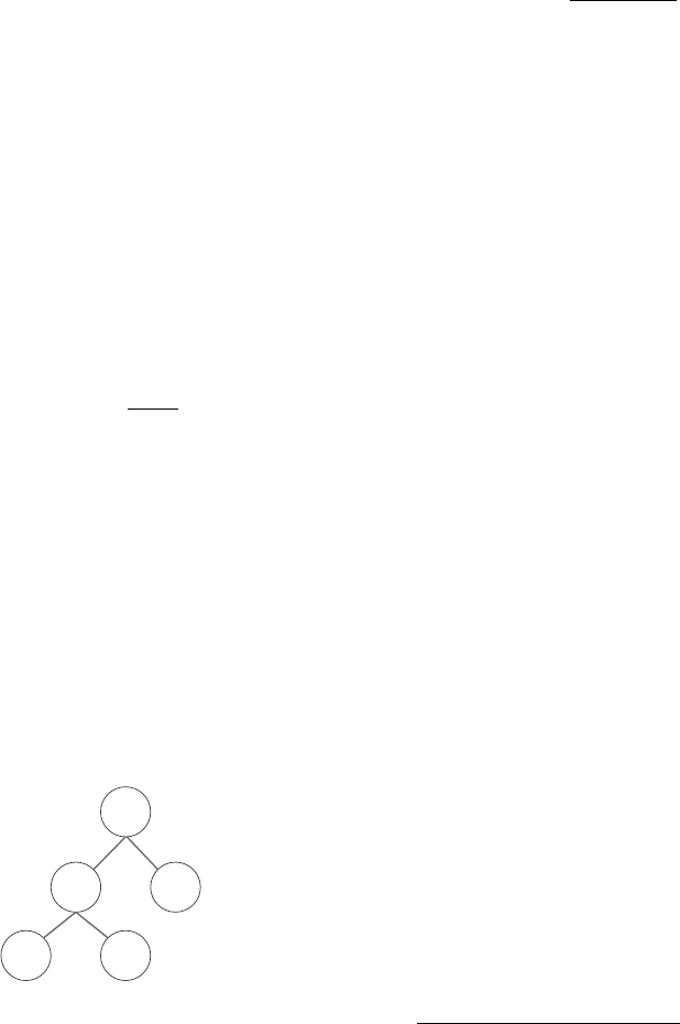
e"
a" b"
d"
c"
Figure 2:
THEOREM 2 Given a set of identical size subgraphs {g
k
} such
that ∪
n
k
g
k
= G
q
, a SJ-Tree with ordered leaves g
k
≺ g
k+1
≺
g
k+2
requires minimal space when f requency(g
k
1 g
k+1
) <
frequency(g
k+2
).
PROOF By induction. Assume a SJ-Tree with three leaves as
shown in Figure 2. Following the definitions of SJ-Tree, this is a
left-deep binary tree with 3 leaves. Therefore, frequency(c) de-
noted in shorthand as f(c) f(c) = min(f(a), f(b)). Substituting
for the frequency of c, space requirement for this tree S(T ) =
f(a) + f(b) + f (d) + min(f(a), f(b)). Thus, the space require-
ment for this tree is minimum if f(a) < f(b) < f(c).
Now we can consider any arbitrary tree where T
n
refers to a tree
with a left subtree T
n
1
and a right child l
n+2
. Above shows that T
1
constructed as above will have minimum space requirement, and so
will T
2
if f(a) < f(b) < f(c) < f(d).
OBSERVATION 3 Given g
k
, a subgraph of query graph G
q
, it is
efficient to decompose g
k
if there is a subgraph g ⊂ g
k
, such that
frequency(g) >
f requency(g
k
)
¯
d|V (g
k
)|
, where
¯
d is the average vertex
degree of the data graph and |V (g
k
)| is the number of vertices in
g
k
.
PROOF Given a graph g, the average cost for searching for an-
other graph that is larger by a single edge is
¯
d multiplied by the
number of vertices in g
k
, and the proof follows.
7. EXPERIMENTAL STUDIES
We present experimental analysis on two real-world datasets (New
York Times
1
and Internet Backbone Traffic data
1
), and a synthetic
streaming RDF benchmark. The experiments are performed to an-
swer questions in the following categories.
1. STUDYING SELECTIVITY DISTRIBUTION What does the se-
lectivity distribution of 2-edge subgraphs look like in real
world datasets? What is the duration of time for which the se-
lectivity distribution or selectivity order of 2-edge subgraphs
remains static?
2. COMPARISON BETWEEN SEARCH STRATEGIES In the pre-
vious sections, we introduced two different choices for query
decomposition (1-edge vs 2-edge path based) and two differ-
ent choices for query execution (lazy vs non-lazy). How do
the strategies compare?
3. AUTOMATED STRATEGY SELECTION Given a dynamic graph
and a query graph, can we choose an effective strategy using
their statistics?
7.1 Experimental setup
The experiments were performed on a 32-core Linux system
with 2.1 GHz AMD Opteron processors, and with 64 GB mem-
ory. The code was compiled with g++ 4.7.2 compiler with -O3
optimization.
Given a pair of data graph and query graph, we perform either of
two tasks: 1) query decomposition and 2) query processing.
Query decomposition: Query decomposition involves loading
the data graph, collecting 1-edge and 2-edge subgraph statistics and
performing query decomposition using the selectivity distribution
of the subgraphs. The SJ-Tree generated by the query decomposi-
tion algorithm is stored as an ASCII file on disk.
Query processing: The query processing step begins with load-
ing the query graph in memory, followed by initialization of the
SJ-Tree structure from the corresponding file generated in the query
1
http://data.nytimes.com
1
http://www.caida.org

decomposition step. We initialize the data graph in memory with
zero edges. Next, edges parsed from the raw data file are streamed
into the data graph. The continuous query algorithm is invoked
after each AddEdge() call to the data graph.
7.2 Data source description
Summaries of various datasets used in the experiments are pro-
vided in Table 1. We tested each dataset with a set of randomly
generated queries. The following describes the individual datasets
and test query generation.
New York Times: The New York Times dataset contains articles
collected from 2013 July-September time period using Version 3 of
its data collection API available at data.nytimes.com. Each
article in the dataset contains a number of facets that belong to
four types of entities: person, geo-location, organization and topic.
Each of the articles and facets are represented as vertices in the
graph. Each edge that connects an article with a facet carries a
timestamp that is the publication time of the article. The New York
Times dataset was tested with a set of 10 randomly generated k-
partite graphs.
Network Traffic The second dataset is an internet backbone traf-
fic dataset obtained from www.caida.org. CAIDA (Coopera-
tive Association for Internet Data Analysis) is a collaborative pro-
gram that provides a wide collection of network traffic data. We
used the “CAIDA Internet Anonymized Traces 2013 Dataset" for
experimentation. The dataset contains 22 million network traffic
flow (subsequently referred to as netflow) records collected over a
one minute period. We excluded the traffic to/from IP addresses
matching patterns 10.x.x.x or 192.168.x.x. These address spaces
refer to private subnets and a communication from a given IP ad-
dress from these spaces can actually refer to multiple physical hosts
in the real word. As an example, every internet service provider
configures the routers or machines inside a home network with IPs
selected from the private IP address range. Therefore, if we see a re-
quest from 192.168.1.1 to google.com, there is no way to determine
the exact origin of this communication. From a graph perspective,
allowing private IP address and the subsequent aggregation of com-
munication will result in the creation of vertices with giant neighbor
lists, which will surely impact the search performance. A detailed
list of use cases describing subgraph queries for cyber traffic mon-
itoring are described in [15].
Social Media Stream Our final test dataset is a synthetic RDF
social media stream available from the Linked Stream Benchmark
(LSBench) [3]. We generated the dataset using the sibgenerator
utility with 1 million users specified as the input parameter. The
generated graph has a static and a streaming component. The static
component refers to the social network with user profiles and so-
cial network relationships. The streaming component includes 3
streams. The GPS stream includes user checkins at various loca-
tions. The Post and Comments stream includes posts and com-
ments by the users, subscriptions by users to forums, and a stream
of “likes" and “tags". Finally, the photo stream includes informa-
tion about photos uploaded by users, and “tags" and “likes" as ap-
plied to photos.
7.3 Selectivity Distribution
Figure 3 shows the edge distribution plotted over time. X-axis
shows the number of cumulative edges in the graph as it is grow-
ing. The plotted distribution is not cumulative. The edge distribu-
tion is collected after fixed intervals. The interval is 10 thousand,
100 thousand and 1 million respectively. There are 4, 7, and 45
edge types in these datasets. The first half of the RDF dataset con-
tains data for a simulated social network. The second half contains
simulated data about the activities in the network such as posts, and
checkins at locations The shift in the edge distribution around the
mid point reflects these different characteristics. The key observa-
tion is that the relative order of different types of edges stays similar
even as the graph evolves.
100 200 300 400 500 600
10
0
10
2
10
4
10
6
10
8
10
10
Unique 2−edge path type
Count
(a) Synthetic social data stream in RDF
Figure 4: 2-edge path distribution in each test data set. Each
point on X-axis represents a unique 2-edge path and Y-axis
shows its corresponding count.
There were 14, 62 and 676 unique 2-edge paths present in the
New York Times, netflow and LSBench datasets. Figure 4 shows
the 2-edge path distribution for the LSBench dataset. We found
a small number of 2-edge subgraphs to dominate the distribution
across all the datasets. Other datasets show a similarly skewed dis-
tribution, and was omitted for space. The skew is heaviest for the
LSBench dataset, which is expected given the higher number of
unique edge types and the larger size of the dataset.
The goal of this analysis was to observe the variability in the
selectivity distribution over time. The selectivity distribution is ex-
pected to vary over time. However, it is the relative order of the
unique single edge or 2-edge subgraphs that matters from the query
decomposition perspective. For each of the test datasets, we took
multiple snapshots of the selectivity order and found it to be stable,
except with fluctuations for the very low frequency components
(data points on the left end of the distributions in Fig. 4). Sig-
nificant changes in the selectivity order can adversely impact the
performance of the query. Estimating the duration over which the
selectivity ordering stays stable for a given data stream, quantifi-
cation of errors based on shift in the distribution, and adapting the
query algorithm to handle such shifts is reserved for future work.
7.4 Query Performance Analysis
This section presents query performance results obtained through
query sweeps on each of the three datasets. For each query, we
collect performance from 4 different query execution strategies ob-
tained by 1-edge or 2-edge decomposition of a query graph and the
lazy vs. track everything approach adapted by the query algorithm.
The following tags are used to describe the plots in the remain-
der of the paper: a) “Single": 1-edge decomposition, search tracks
all matching subgraphs in SJ-tree, b) “SingleLazy": 1-edge based
query decomposition, use “Lazy" approach to search, c) “Path":
2-edge decomposition, search tracks all matching subgraphs in SJ-
Tree, and d) “PathLazy": 2-edge decomposition with “Lazy" search.
7.4.1 New York Times
We begin with our analysis on New York Times (NYT) data. Ten
query graphs were generated using the template as shown in Figure
5. Type of vertices 1 and 2 were kept fixed as “articles", whereas the
type of vertices 3 and 4 were permuted between author, location,
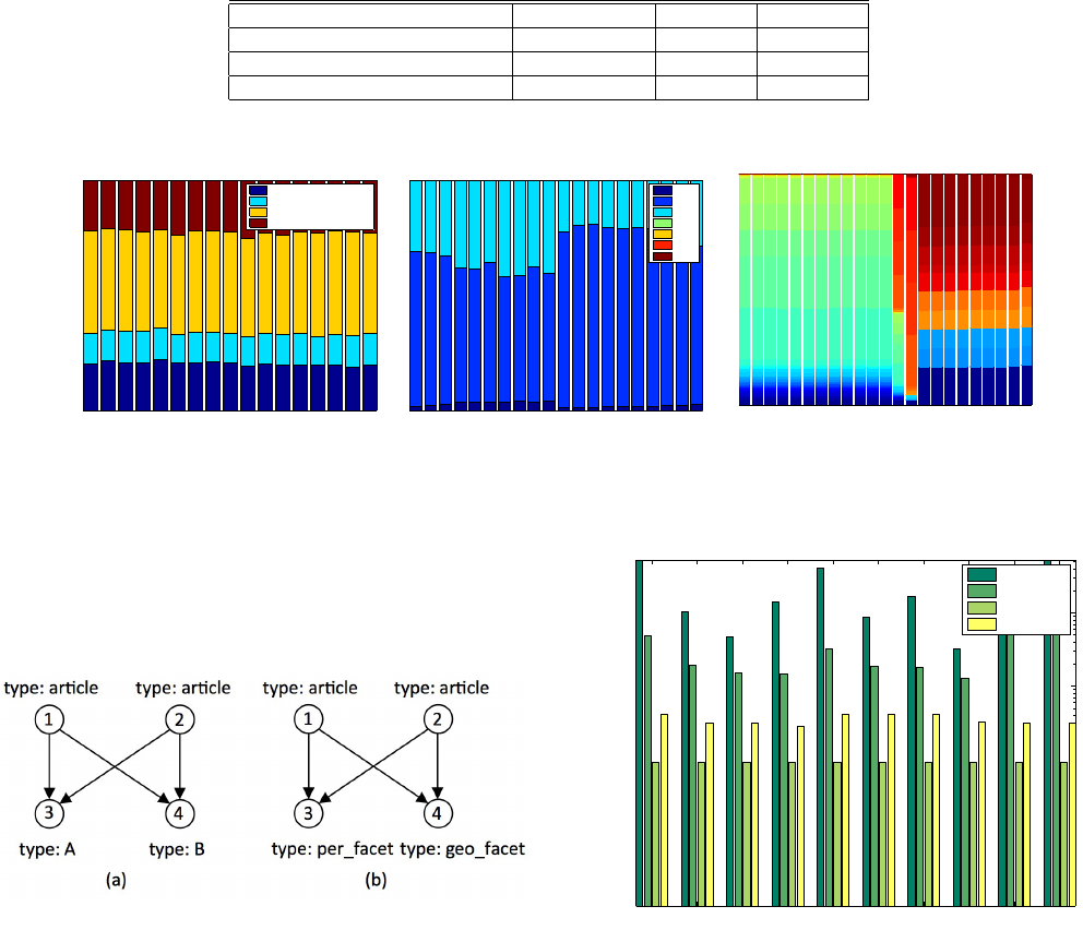
Table 1: Summary of test datasets
Dataset Type Vertices Edges
New York Times Online News 64,639 157,019
Internet Backbone Traffic Network traffic 2,491,915 19,550,863
LSBench/CSPARQL Benchmark RDF Stream 5,210,099 23,320,426
2 4 6 8 10 12 14 16
x 10
4
0
1000
2000
3000
4000
5000
6000
7000
8000
9000
10000
Edge Distribution Over Time
article_mentions_person
article_mentions_geoloc
article_mentions_topic
article_mentions_org
(a) Online news - New York Times
0.2 0.4 0.6 0.8 1 1.2 1.4 1.6 1.8 2
x 10
6
0
1
2
3
4
5
6
7
8
9
10
x 10
4
Edge Distribution Over Time
ICMP
TCP
UDP
IPv6
AH
ESP
GRE
(b) Internet Backbone Traffic - CAIDA
0.5 1 1.5 2
x 10
7
0
1
2
3
4
5
6
7
8
9
10
x 10
5
Edge Distribution Over Time
(c) Synthetic social data stream in RDF
Figure 3: Edge type distribution shown with the evolution of the dynamic graph.
organization and topic. The edge types were also changed to keep
them consistent with the types of end-point vertices. For example,
setting vertex 3 as “author" from “location" required setting the
edge (1, 3) type to “has-author" (from “has-location").
Figure 5: Query template for New York Times.
Figure 6 shows the total run time for processing 100,000 edges
using each of these strategies. Evidently, the "SingleLazy" strategy
that combines lazy-search with 1-edge based decomposition is the
best performing strategy. We were surprised by the “PathLazy" ap-
proach taking a disproportionate amount of time. We discovered
that for most of these queries, the “PathLazy" approach resorted to
searching for a “twig" graph (example: an article connected to a
person and a topic) and once it was found, it spawned off a search
for another twig graph from all the matching vertices. There are
many high-degree vertices in the non-article (geo-location, organi-
zation, person, topic) category. Therefore, any time the search finds
a match around a high degree vertex such as “geo-location:New
York" or “topic:Polictics and Government", it performs a second
search. The high runtime of “PathLazy" results from a large num-
ber of occurrences of this event. While these are insights drawn
from deep analysis into the data, is there a generic way to deter-
mine which might be a better performing strategy? We provide an
answer in section 7.5.
Next, we investigate the relative performance of these strategies
1 2 3 4 5 6 7 8 9 10
10
0
10
1
10
2
10
3
10
4
k−Partite Query Graph ID
Runtime (milliseconds)
PathLazy
Path
SingleLazy
Single
Figure 6: Query processing times using four different search
strategies for New York Times data.
in more detail by studying the individual decompositions and de-
gree distribution. As we discussed in the time complexity analysis
(section 4.1), the subgraph isomorphism cost for single edges is
O(1) and O(
¯
d) for 2-edge subgraphs, where
¯
d is the average de-
gree of the target vertex v
2
in the query subgraph. To verify this, we
plotted the ratio between the “Path" and “Single" strategies (Fig-
ure 7). For the 2-edge or path based decomposition, 8 out of 10
queries were searching for a 2-edge subgraph that has an article
vertex and other the two vertices chosen from the following com-
binations: topic and topic, organization and organization, person
and person, geo-location and geo-location, topic and organization,
topic and person, topic and geo-location, organization and person.
Two of the remaining decompositions resulted in searching for a 2-
edge subgraph that has a person connected to two distinct articles,
or a geo-location connected to two distinct articles. The average
10
0
10
1
1
2
3
4
5
6
7
8
9
10
Ratio of run times (Path/Single)
k−Partite Query Id
10
−3
10
−2
3.2
3.4
3.6
3.8
4
4.2
4.4
Edge Selectivity
Ratio of run times (Single/SingleLazy)
Figure 7: Analyzing relative performance between the top-3
search strategies for New York Times data. X-axis on the lower
plot shows Expected Selectivity measured from edge distribu-
tion data.
degree for vertices of type “article" is 4.03. As Figure 7 shows, the
speedup from “Path" to “Single" closely approximates the average
degree of article vertices, as predicted in the complexity analysis.
Next, we observe the impact of adopting the Lazy approach for
the “Single" strategy. The lower plot in Figure 7 shows the speedup
from Lazy Search as a function of Expected Selectivity computed
from edge distribution. The speedup is seen to be higher with
higher expected selectivity. The expected selectivity is higher if
the probability of individual edges appearing in the graph stream
is high. However, the probability of an edge’s appearance in the
graph stream does not provide us with any information about the
presence of the query match. Given the lazy approach guarantees
the savings in search time, and consequently, reduces the number
of partial matches being tracked, the savings are higher when the
likelihood of the appearance of individual edges in the graph stream
is high.
7.4.2 Network Traffic and LSBench
We present the results from the Netflow and LSBench dataset
in this subsection. Both of these datasets are orders of magnitude
larger than New York Times and the scale allows us to magnify the
differences between multiple strategies.
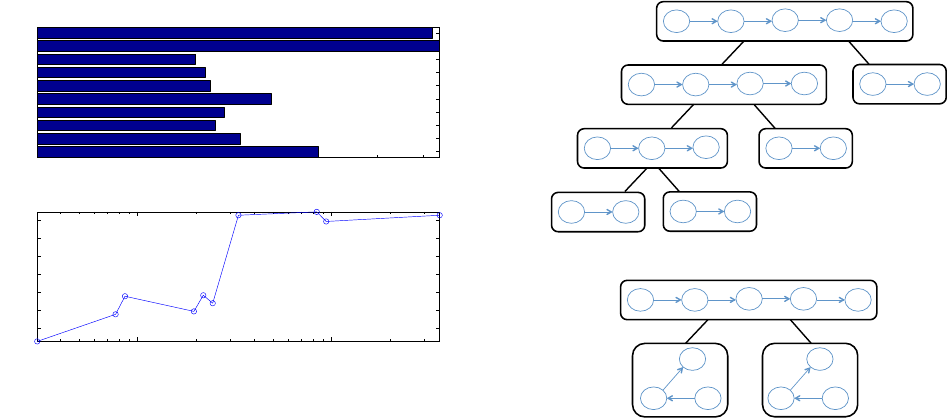
QUERY GENERATION We generate both path queries and binary
tree queries for the netflow data. Figure 8 shows two decompo-
sitions of an example query. The vertex labels are fixed to type
“ip" and the edge types are randomly chosen from a set of 7 pro-
tocols: ICMP, TCP, UDP, IPv6, AH, ESP and GRE. The binary
tree queries were generated following the test generation method-
ology described in [21]. The LSBench dataset is tested with path
queries and n-ary trees. A list of valid triples (vertex type, edge
type , vertex type) is generated using the LSBench schema. A tree
query is generated by randomly selecting an edge from the set of
valid triples and then iteratively adding valid new edges from any
of the nodes available. All our query graphs are unlabeled. Using
netflow data as an example, we do not generate a query that has a
label associated with any of the nodes. In practice, we expect users
to employ labeled queries such as finding a tree pattern in the net-
work traffic where the root of the tree has a IP address (i.e. label)
ip# ip#
ip# ip#
ip#
ESP# TCP#
ICMP#
GRE#
ip# ip#
ip# ip#
TCP# ICMP#
GRE#
ip# ip#
ip#
ICMP# GRE#
ip# ip#
GRE#
ip# ip#
ICMP#
ip# ip#
TCP#
ip# ip#
ESP#
(a)
ip# ip#
ip#
TCP#
ESP#
ip# ip#
ip#
GRE#
ICMP#
ip# ip#
ip# ip#
ip#
ESP# TCP#
ICMP#
GRE#
(b)
Figure 8: 1 and 2-edge based decompositions of a path query
on netflow traffic data.
from a certain subnet. For social data, we may look for paths with
specified user ids (node labels) on the source and the destination
nodes on the path. The impact of the selectivity of labels on query
processing is explored in our previous work [6]. Here, our experi-
ments are motivated to study the impact of subgraph distributional
statistics on query processing.
COMPARISON WITH OTHER APPROACHES In our previous work
[6] we had compared the performance of our implementation with
the IncIsoMatch algorithm proposed by Fan et al. [10]. Our IncI-
soMatch implementation was based on a variant of the well-known
VF2 algorithm [9]. Here, we compare our incremental algorithms
with a non-incremental approach that performs subgraph isomor-
phism for the query graph (using VF2) on every new edge in the
dynamic graph.
SUMMARIZATION OF RESULTS Unlike the New York Times
dataset, where we reported the performance for each randomly gen-
erated query, we present aggregated results for each query group.
All queries of the same type (path or tree) and size (3-hop length or
5 nodes) are denoted as a group. We generated 100 queries for each
group and then eliminated ones that contained 2-edge paths not
seen in the sampled path distribution. This was done for two rea-
sons; first, inclusion of an unseen 2-edge path combination makes
the query artificially discriminative. Our goal is to observe query
processing time as a function of varying selectivity, so including
unusually discriminative queries bias our studies. Second, when
asked to generate a path-based decomposition, our SJ-Tree gener-
ator resorts to generating a single-edge based decomposition when
a query subgraph contains an unseen 2-edge path. This would bias
our comparison between a path-based decomposition and single-
edge based decomposition. Finally, for all the “valid" queries we
further sampled them by the Expected Selectivity computed using
2-edge path distribution and reduced each group to a smaller set
of queries that provide a near uniform sampling of the Expected
Selectivity from the larger set. Finally, the reported runtime for a
given strategy (e.g. “PathLazy") is obtained by averaging the run-
times from the reduced set of queries,
Figure 9a-d shows the query processing times collected for both
3 4 5
10
0
10
1
10
2
10
3
10
4
Path Query Size (Path length)
Runtime (seconds)
Path
Single
PathLazy
SingleLazy
VF2
(a) Runtime for Path Queries on Netflow data.
5 6 7 8 9 10 11 12 13 14 15
10
0
10
1
10
2
10
3
Tree Query Size (Number of Vertices)
Runtime (seconds)
Path
Single
PathLazy
SingleLazy
VF2
(b) Runtime for Tree Queries on Netflow data.
3 4 5
10
0
10
1
10
2
10
3
Path Query Size (Path Length)
Runtime (seconds)
Path
Single
PathLazy
SingleLazy
VF2
(c) Runtime for Path Queries on LSBench data.
3 4 5 6 7 8
10
0
10
1
10
2
10
3
10
4
Tree Query Size (Number of Vertices)
Runtime (seconds)
Path
Single
PathLazy
SingleLazy
VF2
(d) Runtime for Tree Queries on LSBench data.
Figure 9: Runtimes from Path and Tree Queries on Netflow
and LSBench.
−10 −8 −6 −4 −2 0 2
0
2
4
6
New York Times
−10 −8 −6 −4 −2 0 2
0
5
10
Netflow
−10 −8 −6 −4 −2 0 2
0
10
20
30
LSBench
Figure 10: Distribution of Relative Selectivity across queries
with 4 edges in 3 datasets. Relative selectivity is shown on X-
axis in log scale.
datasets. The size of the query processing window was fixed at
8M triples, and the performance statistics were collected at at the
middle and at the end of the graph stream. We profiled different
components of the query processing such as the time spent in per-
forming subgraph isomorphism and the time spent in updating the
SJ-Tree. The latter is largely composed of the time spent in looking
up the hash tables in various nodes of the SJ-Tree, performing joins
between partial matches and inserting new entries. We found that
the subgraph isomorphism operation (for 1 or 2-edge subgraphs)
dominates the processing time. Considering both classes of queries
with diameter 4 and 5, the subgraph isomorphism operation con-
sumes more than 95% of the total query processing time.
A general observation is that the performance of non-incremental
search by VF2 is found to be 10-100x slower. The Y-axis is plot-
ted in log scale, and we can see how the run times of the “Path"
and “Single" approaches rise exponentially as the query sizes are
increased. Overall, we find the “SingleLazy" and “PathLazy" are
the best performing search approaches. As the tree queries show,
the growth rate in the query processing time is much slower for the
“Lazy" variants. This conclusively demonstrates the effectiveness
of restricting the search to where a match is emerging, and growing
the match by starting from the most selective sub-query.
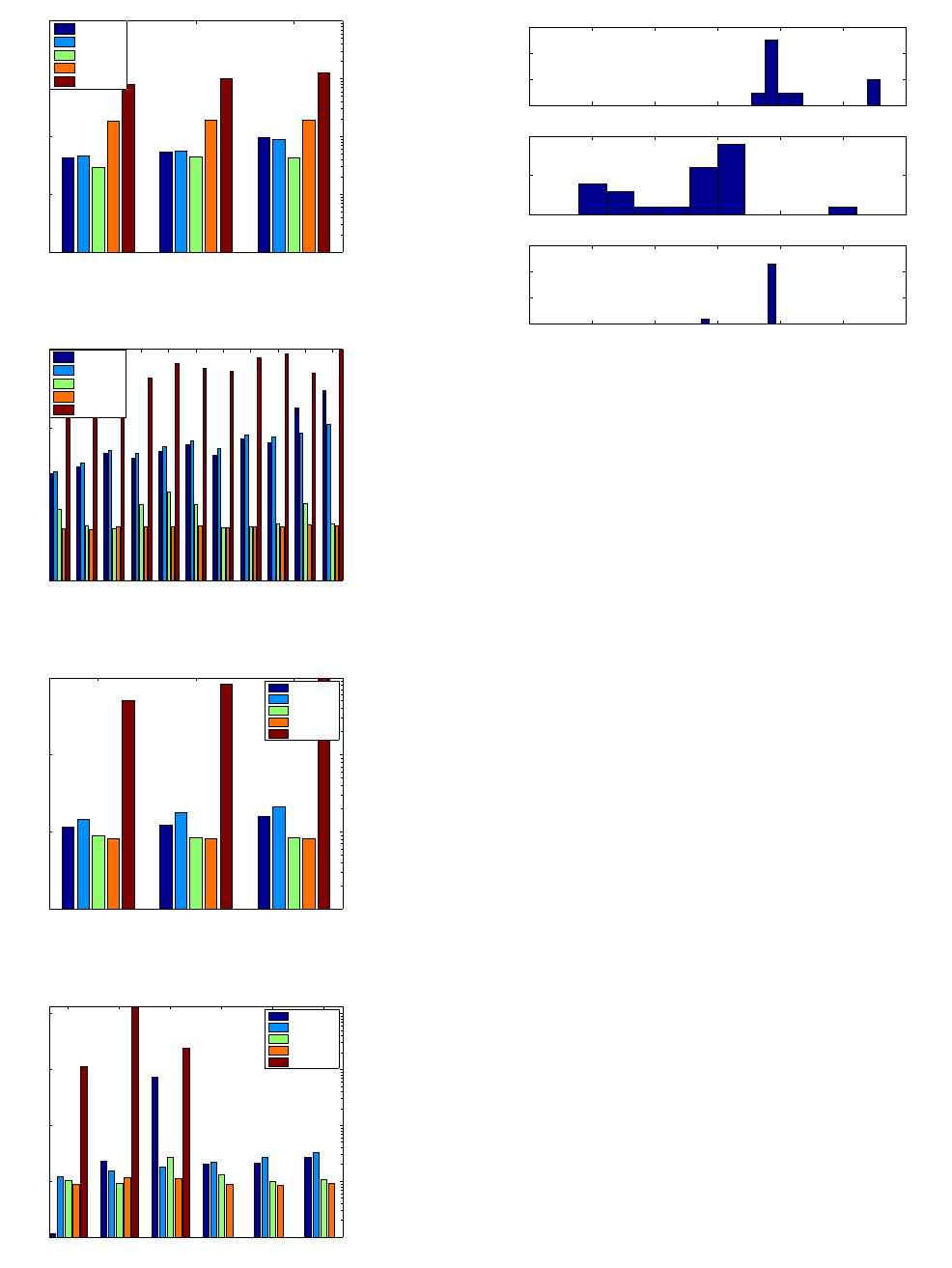
7.5 Analysis via Relative Selectivity
Figure 10 shows the distribution of relative selectivity for queries
with 4 edges across all three datasets. We picked query graphs with
4 edges to find a common basis for comparing different type of
queries (k-partite vs. path queries) across multiple datasets, and the
discussion is equally applicable to larger or different query class
combinations. The top subplot shows the relative selectivity of
10 k-partite queries from the New York Times data. For netflow
and LSBench, we randomly sampled 25 queries from the randomly
generated path query collection. As can be seen, the relative selec-
tivity is very low for the netflow dataset. Following the definition of
relative selectivity, its value is lowered when the path distribution
based selectivity is low. In other words, there are some paths in the
query which have very low probability of occurrence. Therefore,
the “PathLazy" approach is superior for such queries. Empirical
observation on larger path queries and other tree queries seem to
suggest two prominent clusters of relative selectivity values. The
first one typically ranges from 0.001 and above, and the second
one contains values that are smaller by multiple orders of mag-
nitude. This suggests a heuristic that “PathLazy" strategy could
be employed for queries with relative selectivity below 0.001, and
“SingleLazy" be employed for queries above 0.001.
8. CONCLUSION AND FUTURE WORK
We present a new subgraph isomorphism algorithm for dynamic
graph search. We developed a new data structure named Subgraph
Join Tree (SJ-Tree) that represents the execution strategy for a query.
We also developed a set of algorithms for efficient collection of
graph stream statistics, and using the statistics for automatic gener-
ation of the SJ-Tree for any given query graph. We also introduced
two selectivity metrics to quantitatively measure the hardness of a
query by considering the temporal properties of the graph. Given
a stable distribution of edge types and the skew in the distribution
of 2-edge subgraphs, we demonstrated that a query decomposition
based on more selective edges will be consistently efficient. We
went further to introduce a “Lazy" variant of the dynamic graph
search algorithm that exploits the varying selectivity between dif-
ferent parts of a query graph. We also extensively compared dif-
ferent search strategies, performing experiments on three different
datasets and multiple query classes. Finally, we concluded with a
Relative Selectivity based rule for selecting a search strategy.
The paper investigates the important problem of estimating se-
lectivity of query graphs. While our 2-edge subgraph based ap-
proach provides an initial foundation, deeper investigations are war-
ranted for more accurate selectivity estimation. Subsequent re-
search can leverage on the significant body of work on counting
larger subgraphs such as triangles in streaming or semi-streaming
scenarios. Exploring query graphs with more diverse structures
and developing a predictive model for accurate estimation of per-
formance needs to be addressed. Adaptive query processing is an
important follow-up problem as well. A long standing database
query needs to be robust against shift in the data characteristics.
While we propose a fast algorithm for periodic recomputation of
the primitive distribution, we do not address the issues of modeling
the inefficiency from operating under a different selectivity order
and migrating existing partial matches from one SJ-Tree to another.
Acknowledgment
Presented research is based on work funded under the Center for
Adaptive Supercomputing Software - Multithreaded Architecture
at the US Department of Energy’s Pacific Northwest National Lab-
oratory, which is operated by Battelle Memorial Institute.
9. REFERENCES
[1] A. Arasu, B. Babcock, S. Babu, M. Datar, K. Ito,
I. Nishizawa, J. Rosenstein, and J. Widom. Stream: The
stanford stream data manager. In SIGMOD ’03.
[2] B. Babcock, S. Babu, M. Datar, R. Motwani, and J. Widom.
Models and issues in data stream systems. PODS ’02.
[3] D. F. Barbieri, D. Braga, S. Ceri, E. D. Valle, and
M. Grossniklaus. C-sparql: a continuous query language for
rdf data streams. Int. J. Semantic Computing, 4(1), 2010.
[4] S. Chandrasekaran, O. Cooper, A. Deshpande, M. J.
Franklin, J. M. Hellerstein, W. Hong, S. Krishnamurthy,
S. R. Madden, F. Reiss, and M. A. Shah. Telegraphcq:
continuous dataflow processing. SIGMOD ’03.
[5] L. Chen and C. Wang. Continuous subgraph pattern search
over certain and uncertain graph streams. IEEE Trans. on
Knowl. and Data Eng., 22(8):1093–1109, Aug. 2010.
[6] S. Choudhury, L. Holder, G. Chin, and J. Feo. Fast search for
multi-relational graphs. ACM SIGMOD Workshop on
Dynamic Network Management and Mining, 2013.
[7] S. Choudhury, L. Holder, G. Chin, A. Ray, S. Beus, and
J. Feo. Streamworks: A system for dynamic graph search.
SIGMOD ’13.
[8] D. Conte, P. Foggia, C. Sansone, and M. Vento. Thirty years
of graph matching in pattern recognition. Intl. Journal of
Pattern Recognition and Artificial Intelligence, 2004.
[9] L. Cordella, P. Foggia, C. Sansone, and M. Vento. A (sub)
graph isomorphism algorithm for matching large graphs.
IEEE Trans. on Pattern Analysis and Machine Intelli., 2004.
[10] W. Fan, J. Li, J. Luo, Z. Tan, X. Wang, and Y. Wu.
Incremental graph pattern matching. SIGMOD ’11, 2011.
[11] W.-S. Han, J. Lee, and J.-H. Lee. Turboiso: Towards ultrafast
and robust subgraph isomorphism search in large graph
databases. SIGMOD ’13.
[12] H. He and A. K. Singh. Closure-tree: An index structure for
graph queries. ICDE ’06.
[13] J. M. Hellerstein and M. Stonebraker. Predicate migration:
Optimizing queries with expensive predicates, volume 22.
ACM, 1993.
[14] M. Jha, C. Seshadhri, and A. Pinar. A space efficient
streaming algorithm for triangle counting using the birthday
paradox. In SIGKDD. ACM, 2013.
[15] C. Joslyn, S. Choudhury, D. Haglin, B. Howe, B. Nickless,
and B. Olsen. Massive scale cyber traffic analysis: a driver
for graph database research. In 1st ACM SIGMOD Workshop
on Graph Data Management Experiences and Systems, 2013.
[16] A. Khan, N. Li, X. Yan, Z. Guan, S. Chakraborty, and S. Tao.
Neighborhood based fast graph search in large networks.
SIGMOD ’11.
[17] R. Krishnamurthy, H. Boral, and C. Zaniolo. Optimization of
nonrecursive queries. In VLDB, volume 86, pages 128–137.
Citeseer, 1986.
[18] Y.-N. Law, H. Wang, and C. Zaniolo. Relational languages
and data models for continuous queries on sequences and
data streams. ACM Trans. Database Syst., June 2011.
[19] J. Mondal and A. Deshpande. Eagr: Supporting continuous
ego-centric aggregate queries over large dynamic graphs. In
SIGMOD 2014.
[20] C. Seshadhri, A. Pinar, and T. G. Kolda. Fast triangle
counting through wedge sampling. In Proceedings of the
SIAM Conference on Data Mining, 2013.
[21] Z. Sun, H. Wang, H. Wang, B. Shao, and J. Li. Efficient
subgraph matching on billion node graphs. PVLDB, 5(9),
2012.
[22] Y. Tian and J. Patel. Tale: A tool for approximate large graph
matching. In ICDE ’08.
[23] H. Tong, C. Faloutsos, B. Gallagher, and T. Eliassi-Rad. Fast
best-effort pattern matching in large attributed graphs. KDD
’07.
[24] J. R. Ullmann. An algorithm for subgraph isomorphism. J.
ACM, 23:31–42, January 1976.
[25] Y. Wu, J. M. Patel, and H. Jagadish. Structural join order
selection for xml query optimization. In Data Engineering,
2003. Proceedings. 19th International Conference on, pages
443–454. IEEE, 2003.
[26] P. Zhao, C. C. Aggarwal, and M. Wang. gsketch: on query
estimation in graph streams. PVLDB, 5(3), 2011.
[27] P. Zhao and J. Han. On graph query optimization in large networks. PVLDB., 3:340–351, September 2010.
