1
Tsunami risk and information shocks: Evidence from the Oregon
housing market
Amila Hadziomerspahic
1
Oregon State University
September 2021
PRELIMINARY DRAFT – PLEASE DO NOT CITE WITHOUT PERMISSION
Abstract: Estimating risk perceptions related to natural disasters is critical to understanding behavioral
responses of individuals and adaptive capacity of communities. Developed coastlines experience hazard
risk from sources with different frequency and intensity, such as flooding, erosion, and sea-level rise. In the
Pacific Northwest, there is an additional high severity but very low frequency risk: the Cascadia Subduction
Zone earthquake and tsunami. This paper investigates the impact of tsunami risk information on coastal
residents’ risk perceptions, as capitalized into property prices, using difference-in-differences and triple
differences hedonic frameworks. I study the coastal Oregon housing market response to three sets of risk
signals: two exogenous events - the March 11, 2011 Tohoku earthquake and tsunami and the July 20, 2015
New Yorker article “The Really Big One”; a hazard planning change – the 2013 release of new official
tsunami evacuation maps; and visual cues of tsunami risk – blue lines indicating the spatial extent of the
hazard zone installed by Oregon’s Tsunami Blue Line project. For the first analysis, results suggest that a
property inside the primary tsunami inundation zone sells for 6.5-8.5% less than a property outside of the
zone after the Tohoku event, with a return to baseline levels within 2.5 years. For the second analysis, I find
evidence that the 2013 hazard planning change was capitalized into home values in only the most vulnerable
new inundation zone. For the third analysis, results suggest houses near blue lines may be selling for 8.0%
less compared to houses farther away. The potential risk discounts identified in these analyses suggest that
tsunami risk signals can be salient to coastal residents.
Keywords: Natural hazard risk, tsunamis, hedonic models, difference-in-differences, triple differences
JEL codes: Q51, Q54
This research was supported by Oregon Sea Grant under award no. NA18OAR170072 (CDFA no. 11.417)
from NOAA’s National Sea Grant College Program, US Department of Commerce, and by appropriations
made by the Oregon State Legislature. Housing data provided by Zillow through the Zillow Transaction
and Assessment Dataset (ZTRAX). More information on accessing the data can be found
at http://www.zillow.com/ztrax
. The results and opinions are those of the author and do not reflect the
position of Zillow Group.
1
Ph.D. candidate at Oregon State University, Department of Applied Economics, 322 Ballard Extension Hall, Corvallis, OR 97331.
E-mail: [email protected]
.
2
1 Introduction
Severe but low frequency events pose a unique challenge for hazard planning. The connection between risk
perception about catastrophic events and preparedness action is still much disputed (Wachinger et al.,
2013). The risk of a catastrophic natural disaster must be salient to the people it will impact to translate into
personal preparedness. If the risk is either not salient to individuals or does not translate into behavior
change, it may fall on policymakers to correct the market failure to internalize risk and increase resilience.
The Pacific Northwest of the United States (U.S.) is facing such a challenge. There is a 7 to 15
percent chance for a major earthquake (up to 9.2 in magnitude) to occur in the next 50 years along the
Cascadia Subduction Zone (CSZ) (OSSPAC, 2013). In Oregon, preparedness for such a large seismic event
is low. A recent study estimated that economic losses could be more than $30 billion – almost one-fifth of
Oregon’s gross state product – and fatalities due to the combined earthquake and tsunami could be more
than ten thousand (OSSPAC, 2013). Coastal communities in the tsunami zone are especially vulnerable
since they will experience the strongest earthquake motions due to their proximity to the fault, will be
subject to multiple tsunami inundations, and will account for the majority of expected fatalities (OSSPAC,
2013; Schulz, 2015b).
Individual Oregonians can increase their resilience by retrofitting their homes, purchasing
earthquake and flood insurance, or moving away from high-risk areas such as the tsunami inundation zone.
Whether individuals will take action to prepare themselves depends in part on their beliefs about the risk of
a Cascadia earthquake and tsunami occurring in their lifetimes. If Oregonians’ subjective risk perceptions
underestimate the objective probability of a Cascadia event – if the risk is not salient – then they will likely
underprepare themselves. This gap between subjective risk perceptions and objective risk is plausible given
that Oregon has not experienced a major earthquake and tsunami in recent history – the last CSZ earthquake
and tsunami occurred in 1700 – and has low resilience compared to countries, like Japan and Chile, that
regularly experience earthquakes (OSSPAC, 2013). The lack of recent earthquakes has led Oregon to also
be less prepared and more vulnerable than its neighboring states of California and Washington (Totten,
2019). This motivates an important question about tsunami risk perceptions: Can new information about
the risk of a Cascadia earthquake and tsunami change people’s risk perceptions and narrow the gap between
subjective and objective risk? Here, I investigate whether a risk discount is present in coastal Oregon
housing markets following exogenous information shocks about tsunami risk. I study the housing market’s
response to three sets of risk signals: 1) two exogenous events – the March 11, 2011 Tohoku (Japan)
earthquake and tsunami and the July 20, 2015 New Yorker article “The Really Big One”; 2) a hazard
planning change – the release of new official tsunami evacuation maps in 2013 by the Oregon Department
of Geology and Mineral Industries (DOGAMI); and 3) visual cues of tsunami risk – the Tsunami Blue Line
3
project, which installed signage denoting the upper limit of the tsunami inundation zone in communities
along the coast.
Using a dataset of residential property transactions for the Oregon coast (Zillow, 2020), I estimate
the treatment effects of these tsunami risk signals in a series of hedonic difference-in-differences (DID) and
triple differences (DDD) frameworks. First, I use information from the northern Oregon coast housing
market to estimate the impact of two exogenous events that represent “pure” or “distant” information shocks
in that there is no actual disaster event or that the disaster event is distant and there is little associated local
damage. An increased volume of Google searches suggest that these events were salient to Oregonians and
may be a mechanism by which individuals update perceptions of risk related to the potential for a major
Cascadia event. I test how these information shocks capitalize into home values in the three northernmost
coastal counties in Oregon (Clatsop, Tillamook, and Lincoln). I differentiate risk using a regulatory tsunami
hazard line as the treatment boundary since the entire coastline is likely to face similar impacts from an
earthquake. Results suggest that a property inside the regulatory tsunami inundation zone sells for 6.5 -
8.5% less than a property outside of the zone after the Tohoku event. This result is robust to a number of
alternative specifications, including the Oaxaca-Blinder estimator, four post-matching estimators, and an
event study specification. I find that the effect is short-lived as property prices inside the inundation zone
quickly return to baseline levels within 2.5 years of the Tohoku event.
I then use housing information from the entire Oregon coast to estimate the impact of the 2013
update of official tsunami inundation and evacuation maps based on a new series of modeled inundation
maps for five CSZ scenarios (S, M, L, XL, XXL) (DOGAMI, n.d.-a). The largest of this series – the XXL
scenario – became the inundation line for official tsunami evacuation brochures and signage, supplanting
the original and more conservative inundation line that was established in 1995 through Senate Bill 379.
This hazard planning change represents a tsunami risk signal – and a “pure” information shock – about
houses that were not in the original 1995 SB 379 evacuation zone but found themselves inside one of the
new 2013 inundation zones. I find the estimates are not statistically significant for the XXL, XL, L or M
tsunami inundation zones. The DID and Oaxaca-Blinder estimators for the smallest inundation zone (SM)
suggest that homes that were not in the original tsunami inundation zone but are now in the most vulnerable
inundation zone sell for 17 - 27% less after the map update. This risk discount does not have a statistically
significant decay effect.
Lastly, the Tsunami Blue Line project has installed thermoplastic blue line signs on the 2013 XXL
tsunami inundation line on roads in several coastal communities since its launch in 2016 (Office of
Emergency Management, 2016). The blue lines are visual cues of tsunami risk and their installation
represents a tsunami risk signal and a “pure” information shock to properties near those blue lines. To
determine whether this project resulted in a risk discount for homes near the blue lines and inside the
4
tsunami evacuation zone, I estimate the effect of the blue lines on property prices, with properties
differentiated by proximity to the blue lines and – for a DDD approach – by the XXL tsunami inundation
zone. Results from my preferred standard two-way fixed effects (TWFE) DID model suggest there is an
8.0% risk discount for properties that are within 1000’ of a blue line. The DDD results for this model are
not statistically significant, suggesting homebuyers attend to the visual cue but not the risk signal given by
the tsunami inundation zone. However, since the blue lines were installed at different times, there is
variation in treatment timing. Several recent studies have pointed out problems with interpreting the results
of the standard TWFE DID regression when the treatment effect is heterogeneous over time (Borusyak &
Jaravel, 2017; de Chaisemartin & D’Haultfœuille, 2020; Goodman-Bacon, 2018; Sun & Abraham, 2020).
To explore this further I first assess the robustness of the TWFE estimator to heterogeneous treatment
effects using the measure proposed by de Chaisemartin and D’Haultfœuille (2020) and then I estimate two
new estimators that are valid in the presence of treatment effect heterogeneity (Callaway & Sant’Anna,
2020; de Chaisemartin & D’Haultfœuille, 2020). Using de Chaisemartin's and D’Haultfœuille's (2020)
approach, I find a large, negative, but not statistically significant effect. The data for this analysis is too
sparse to be able to estimate most of Callaway's and Sant’Anna's (2020) group-time average treatment
effects. Treatment effect heterogeneity could be a problem for this analysis, however, this dataset is
composed of small, rural communities so I do not have the power to precisely estimate treatment effects
that account for treatment effect heterogeneity.
This work contributes to the hedonic literature on catastrophic risk and the impacts of information
on subjective risk perceptions. This paper is one of few studies that attempts to measure the effects of “pure”
or “distant” information shocks in that either there is no actual disaster event, as in the case of the 2015
New Yorker article, 2013 evacuation map change, and the Tsunami Blue Line project, or that the disaster
event is distant and there is little associated local damage, as in the case of the 2011 Tohoku earthquake
and tsunami (Atreya & Ferreira, 2015; Brookshire et al., 1985; Gibson & Mullins, 2020; Gu et al., 2018;
Hallstrom & Smith, 2005; Nakanishi, 2017; Parton & Dundas, 2020). To my knowledge, this paper is also
the first to investigate the tsunami risk discount in property values disentangled from the earthquake risk
discount. Previous studies have explored either the combined earthquake and tsunami risk or the earthquake
risk alone (Beron et al., 1997; Brookshire et al., 1985; Gu et al., 2018; Nakanishi, 2017; Naoi et al., 2009).
This study’s results also contribute to the literature on risk salience (Kask & Maani, 1992; Nakanishi, 2017)
and the link between risk perception and preparedness action (Wachinger et al., 2013).
My results have important risk communication and policy implications for the Pacific Northwest.
Research shows that Oregon is chronically under-prepared for a Cascadia earthquake and tsunami
(OSSPAC, 2013). Policymakers and emergency managers will need to communicate risk more effectively
to increase risk salience and induce individual decision-makers to take appropriate preparedness actions.

5
Some recent policy changes have even done the opposite. House Bill 3309, passed and signed in June 2019
with nearly unanimous bipartisan support in both the Oregon House and Senate, overturns a nearly 25-year-
old law prohibiting new schools, hospitals, jails, police stations, and fire stations from being built in the
tsunami inundation zone (Oregonian, 2019). Efforts such as this run counter to Oregon’s dual policy
challenge of increasing risk salience and preparedness actions. The potential risk discounts identified here
suggest that at least three types of tsunami risk signals – exogenous events, hazard planning changes, and
visual cues – may be salient to coastal residents. These results suggest that “pure” or “distant” information
shocks can shift homebuyers’ subjective risk perceptions to better match the objective risks of the Cascadia
event. Thus, according to these findings, policies and other “pure” information shocks may be able to
successfully communicate the risk of a Cascadia event and induce individuals to take preparedness actions.
And given Oregon’s current and chronic under-preparedness for a Cascadia event, additional policies – or
risk signals – are needed to mitigate hazard risk.
This paper proceeds as follows. Section 2 reviews the hedonic literature on risk and hazards, along
with empirical strategies to investigate price differentials across hazard zones and the persistence of risk
premium changes. Section 3 describes the study areas and their policy and news backgrounds. Section 4
describes the data collected and some key data limitations. Section 5 defines my empirical approach and
discusses identification strategies for all three analyses. Section 6 presents results for all three analyses.
Section 7 concludes by providing a summary of my current findings, potential next steps to identify these
risk signals, and implications for resilience planning and policy.
2 Hazards and housing markets: previous research
The property attribute of interest in this paper is subjective tsunami risk and I use hedonic frameworks to
test whether three different types of tsunami risk signals capitalize into coastal Oregon property values.
Rosen's (1974) seminal paper was the first to show that regressing observed product prices on their
attributes can reveal buyers’ marginal willingness-to-pay (MWTP) for individual attributes of a
differentiated product.
2
Modern hedonic property models typically rely on the foundational assumptions
that the total supply of housing is fixed and implicit marginal prices represent market equilibria (Hanley et
2
Kuminoff and Pope (2014) point out that the parameters estimated by panel models such as difference-in-differences are not
necessarily theoretically equivalent to the parameters (MWTP) identified by the reduced-form (first-stage) hedonic model. Rosen’s
model considers market equilibrium, not the equilibrating process that would follow an exogenous change in product attributes. If
we are willing to make the assumption that the gradient of the price function is constant over the duration of the study period, then
we can interpret the panel model coefficients as MWTP values (Kuminoff & Pope, 2014). This is a strong assumption for study
periods that span potentially large changes in house and neighborhood attributes – such as the eight-year duration of the first
analysis (2009-2017). Therefore, I interpret the coefficient estimates from my hedonic approach as capitalization effects, not
MWTP, because they describe how the change in the attribute of interest was capitalized into housing prices over time.
6
al., 2007). Since Rosen (1974), many studies have used this method to estimate capitalization of risk factors
in housing prices.
Previous literature has used hazard events or regulatory hazard delineation to identify the impact
of risk on housing prices. In one of the first studies of its kind, Brookshire et al. (1985) found significant
discounting of housing prices in zones with high earthquake risk in California following the passing of an
earthquake risk disclosure law in 1974. The majority of hedonic earthquake risk studies have examined the
impacts of specific earthquake events (Beron et al., 1997; Gu et al., 2018; Naoi et al., 2009). Other hedonic
studies that investigate earthquake risk impacts without the occurrence of a local seismic event have
nonetheless focused on locations like California and Japan where earthquakes have occurred in recent
memory (Brookshire et al., 1985; Nakanishi, 2017). Hedonic models have also been used to measure risk
premiums for natural hazards like floods (Atreya et al., 2013; Kousky, 2010), hurricanes (Bakkensen et al.,
2019; Bin & Landry, 2013; Gibson & Mullins, 2020; Hallstrom & Smith, 2005), wildfires (McCoy &
Walsh, 2018), and coastal storm surge (Dundas, 2017; Qiu & Gopalakrishnan, 2018), as well as man-made
sources of risk like proximity to fuel pipelines (Hansen et al., 2006) and hazardous waste sites (McCluskey
& Rausser, 2001).
Recently, difference-in-differences (DID) approaches have been used to show that disaster events
can increase house price differentials across hazard zones (Atreya et al., 2013; Bakkensen et al., 2019; Bin
& Landry, 2013; Gibson & Mullins, 2020; McCoy & Walsh, 2018; Nakanishi, 2017; Naoi et al., 2009).
The quasi-experimental DID approach uses a recent disaster as an exogenous information change to
separate properties into a treatment group that experiences the disaster event and a control group that does
not. The idea behind this approach is that the disaster event provides new information that causes a change
in the level of subjective risk that may capitalize into house prices. Temporal variation in the attribute of
interest is used to difference out time-invariant omitted variables that would otherwise confound
identification. The DID approach allows us to isolate contemporaneous effects, such as macroeconomic
shocks or housing supply changes, and measure only the effect attributable to the exogenous risk signal.
Triple differences (DDD) has also been used to recover amenity and disamenity effects on property prices
(Bakkensen et al., 2019; Muehlenbachs et al., 2015; Qiu & Gopalakrishnan, 2018). In the hazard risk
literature, the DDD approach has typically exploited an additional treatment (control) group that is more
(less) sensitive to the treatment, i.e., the DDD estimator compares the DID estimator for observations
considered to be more sensitive to the treatment to the DID estimator for observations that are less sensitive
to the treatment.
Information available to housing market participants can change due to a catastrophic event, media
coverage, or new laws (Bakkensen et al., 2019; Bin & Landry, 2013; Brookshire et al., 1985; Gibson &
Mullins, 2020; Hallstrom & Smith, 2005; Kask & Maani, 1992; Kousky, 2010; McCluskey & Rausser,
7
2001; McCoy & Walsh, 2018; Parton & Dundas, 2020; Qiu & Gopalakrishnan, 2018). Kask and Maani
(1992) were the first to show that consumers’ subjective probabilities may under or overestimate objective
probabilities, biasing hedonic prices under conditions of uncertainty. Under the uncertainty of a hazardous
event occurring, hedonic prices are based on consumers’ subjective probability which they define as a
function of the objective probability, the consumer’s expenditures on self-protection (e.g., insurance) and
information level (an exogenous variable). The effect of increased information on behavior depends on the
gap between objective risk and the consumer’s initial subjective risk, e.g., above-average objective risk and
a lower initial subjective probability will lead to increasing subjective probability and hedonic price as
information increases (Kask & Maani, 1992).
New information can lead individuals to update their subjective perceptions of risk and, in turn,
risk premiums may be identified in a hedonic model. However, few studies have attempted to measure the
effects of a “pure” information shock – when there is no actual disaster event – on property prices (Atreya
& Ferreira, 2015; Brookshire et al., 1985; Gibson & Mullins, 2020; Nakanishi, 2017; Parton & Dundas,
2020). For example, Gibson and Mullins (2020) use DID to look at housing market responses to two “pure”
flood risk signals in New York – the passing of the Biggert-Waters Flood Insurance Reform Act (which
increased flood insurance premiums) and new floodplain maps produced by the Federal Emergency
Management Agency (FEMA) – as well as housing market responses to an actual disaster event – Hurricane
Sandy. The release of the new floodplain maps, which had not been updated in 30 years, was accompanied
by prominent press coverage and presented New Yorkers with three decades worth of updated information
about climate change in a single event. Hurricane Sandy and the Biggert-Waters Act, similarly, acted as
exogenous information shocks about flood risk. Gibson and Mullins (2020) find that all three flood risk
signals decreased the sales prices of impacted properties by 3% to 11% (depending on the risk signal).
Furthermore, salience of risk may capitalize into property prices only temporarily after a disaster
event. Other studies have found that the change in risk premium due to a disaster event may disappear
rapidly over the course of a couple of years if additional disaster events do not occur (Atreya et al., 2013;
Bin & Landry, 2013; Hansen et al., 2006; Kousky, 2010; McCluskey & Rausser, 2001; McCoy & Walsh,
2018). Leveraging multiple storm events in North Carolina, Bin and Landry (2013) find risk premiums
between 6.0% and 20.2% following major flooding events for properties inside the 100-year flood zone.
This risk premium decreases over time without new flood events and disappears 5-6 years after the last
recorded event. This decay of risk premium suggests that people’s risk perceptions change with the
prevalence of disaster events. Without new information, individuals’ subjective probabilities will diminish.
Hansen et al. (2006) investigate the effects of distance from a fuel pipeline on property prices in Bellingham,
WA before and after a major pipeline accident in 1999. They find a large risk discount following the
accident and that, for a given distance from the pipeline, the effect of the explosion decays over time.
8
Hansen et al. (2006) point out three reasons why the effect of an event on subjective risk perceptions may
decrease over time. First, the informational effect of the event will diminish as new people move into the
area. Second, individuals who were exposed to the event may experience decay of their active recall.
Finally, as media coverage decreases and people’s attention turns to more recent events, the attention-
focusing effect of the event will diminish over time.
Another potential explanation for the observed decay in risk premium over time is availability bias
– wherein individuals’ subjective probability of an event occurring depends on how recent or memorable
that event was (Atreya et al., 2013; Bin & Landry, 2013; Gallagher, 2014; Kousky, 2010; McCoy & Walsh,
2018). For example, Gallagher (2014) uses an event study framework to estimate the effect of large regional
floods on insurance uptake rates and finds strong evidence of an immediate increase in the fraction of
homeowners with flood insurance policies in communities hit by the flood. The insurance uptake rate
steadily declines until, after nine years, the effect of the flood is no longer statistically distinguishable in
uptake rates. Gallagher (2014) also finds that this insurance uptake spike-and-decay pattern repeats if a
community is hit by another flood, suggesting that the occurrence of new flood events is relatively important
in forming flood risk beliefs. Without new information, individuals’ subjective probabilities will diminish.
However, even when the natural hazard risk is salient, it may not translate into behavior. In their
review of prior research on natural hazard risk perception and behavior, Wachinger et al. (2013) find that
the link between risk perception and preparedness action can be weak even when individuals understand
the risk. Wachinger et al. (2013) also find that the main factors responsible for determining risk perception
are direct experience of a natural hazard, trust in scientific experts and authorities, and confidence in
protective measures. Secondary but significant factors include media coverage, a form of indirect
experience, and home ownership, which stimulates concern when the homeowner perceives a vulnerability
or has personal experience. They note that the indirect experience provided by mass media influences risk
perception but only when the respondents lack direct experience.
3 Study area and background
Oregon is a geologic mirror image of northern Japan, where the March 11, 2011 magnitude 9.0 Tohoku
earthquake caused widespread damage. The resulting tsunami surges also caused millions of dollars of
damages to parts of the Oregon coast (Jung, 2011). The majority of damage in Oregon was concentrated in
the port of Brookings where the waves destroyed docks, resulting in $7 million in damage (Tobias, 2012).
Longer-term effects of the tsunami included multiple cleanup efforts as debris from Japan slowly made its
way to Oregon shores.
Oregon is due to experience a major subduction zone earthquake of a similar magnitude to the
Tohoku event. The probability of a Cascadia Subduction Zone (CSZ) earthquake occurring in the next 50
9
years is 7-15% for a great earthquake between 8.7 and 9.2 magnitude and approximately 37% for a very
large earthquake between 8.0 and 8.6 magnitude (OSSPAC, 2013). Unlike Japan, Oregon’s resilience to a
magnitude 9.0 Cascadia earthquake is low. Coastal communities in the tsunami zone are especially
vulnerable since they will experience the strongest earthquake motions due to their proximity to the fault
and will then be subject to multiple tsunami inundations for up to 24 hours after the earthquake (OSSPAC,
2013). Residents who live within the tsunami inundation zone may be displaced instantly. It may take 3 to
6 months to restore electricity, 1 to 3 years to restore drinking water, and up to 3 years to restore healthcare
facilities on the coast (OSSPAC, 2013).
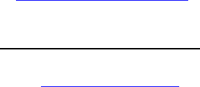
In their 2013 report, the Oregon Seismic Safety Policy Advisory Commission (OSSPAC) (2013)
separated Oregon into four impact zones based on the expected pattern of damage for a 9.0 Cascadia
earthquake and tsunami scenario (Figure 1). They predict that damage will be the most extreme in the
tsunami (inundation) zone and heavy throughout the coastal zone. The coastal zone, which encompasses
most of the coastal county population centers, is expected to experience severe damages from shaking,
liquefaction, and landslides. Throughout the coastal zone, single-family homes and other wood frame
structures will shift off foundations if unsecured. In some areas of the coast, even well-built wooden
structures may be heavily damaged and in need of replacement. However, in the tsunami (inundation) zone,
the damage will be nearly complete. The tsunami will not only further damage buildings, roads, and utilities
but it will also “obliterate nearly all wood frame buildings” (OSSPAC, 2013, p. 49). This difference in
outcomes of residential buildings inside versus outside the tsunami inundation zone suggests that there is a
distinct difference between earthquake and tsunami risk for coastal residents. Similarly, the tsunami zone
will also experience a higher proportion of fatalities. Approximately 4% of permanent residents in the seven
coastal counties live in the tsunami inundation zone (as defined by the 1995 SB 379 regulatory tsunami
line) (Wood, 2007). However, half of the fatalities of a 9.0 magnitude Cascadia event are expected to be
due to the tsunami (OSSPAC, 2013).
Even though the entire coastline would experience similar impacts from an earthquake, coastal
homes outside of the tsunami inundation zone may survive the Cascadia earthquake but those inside of the
zone will likely not. In this paper, I differentiate risk using the tsunami inundation lines from maps produced
by the Oregon Department of Geology and Mineral Industries (DOGAMI) as the treatment boundaries.
Senate Bill 379 established the original tsunami inundation zone in Oregon in 1995. This line, also known
as “SB 379,” represents the best estimate of tsunami inundation from a typical or most likely Cascadia
earthquake in 1995 (DOGAMI, n.d.-b). The 1995 SB 379 line was the regulatory tsunami inundation line
for Oregon until 2019 and limited the construction of certain critical and essential facilities inside the
inundation line (DOGAMI, n.d.-b). House Bill 3309 overturned the regulatory power of the SB 379 line in
2019. Official tsunami evacuation brochures and signage used the SB 379 line until 2013 when DOGAMI
10
released a new series of tsunami inundation maps for a Cascadia earthquake. The 2013 tsunami inundation
map series TIM Plate 1 was derived using systematic, Oregon-coast-wide models of tsunami inundation for
five scenarios – XXL, XL, L, M, and SM – that represent the full range of severity of past and expected
tsunamis (DOGAMI, n.d.-a). The largest scenario of this series – the XXL scenario – became the one used
by DOGAMI to represent the “maximum local source” inundation level in their official tsunami evacuation
maps and signage (DOGAMI, n.d.-a). Thus, the XXL scenario has represented the tsunami evacuation line
for the public at large since 2013. The release of the evacuation maps in 2013 also confronted homeowners
who were outside of the 1995 SB 379 evacuation zone but inside the 2013 XXL evacuation zone with new
and up-to-date information about tsunami risk. Thus, this change in hazard planning also acts as a “pure”
information shock about those houses.
The July 20, 2015 New Yorker article “The Really Big One” by Kathryn Schulz (2015a) brought
national media attention to the predicted Cascadia event and to Oregon’s low level of resilience and
preparation for it. This article went viral in the summer of 2015 (Fletcher & Lovejoy, 2018; Lacitis, 2015;
Marum, 2016). It also prompted preparedness actions such as the selling out of emergency preparedness
kits (Lacitis, 2015; Lovejoy, 2018), earned its author a Pulitzer (Marum, 2016), and motivated a book
addressing risk perception, preparedness, and communication (Fletcher & Lovejoy, 2018). In a chapter of
Figure 1. Impact zones for the magnitude 9.0 Cascadia earthquake scenario. Damage will be extreme in the Tsunami zone,
heavy in the Coastal zone, moderate in the Valley zone, and light in the Eastern zone. From Figure 1.5 of the “Oregon Resilience
Plan” (OSSPAC, 2013).
11
this book, Crowe (2018) compares media coverage of the CSZ before and after Schulz’ article. She finds
that before Schulz’ article the 3 largest spikes in U.S. newspaper coverage occurred after the 2001 Nisqually
earthquake in WA, the 2004 Indian ocean earthquake and tsunami, and the 2011 Tohoku earthquake and
tsunami (Crowe, 2018). The Tohoku earthquake and tsunami had the most media coverage to date that
connects the CSZ to another natural disaster. Within 3 months of “The Really Big One”, 33 unique
newspaper articles were published that referenced both Schulz’ article and the CSZ. Journalists reported on
increased individual actions following the article, e.g., spikes in earthquake survival kit sales and home
earthquake retrofitting, and group actions including public forums, events, and roundtables on earthquake
preparedness. Essentially, “The Really Big One” both communicated the risk of the Cascadia earthquake
and tsunami and spurred the public to prepare for it (Lovejoy, 2018).
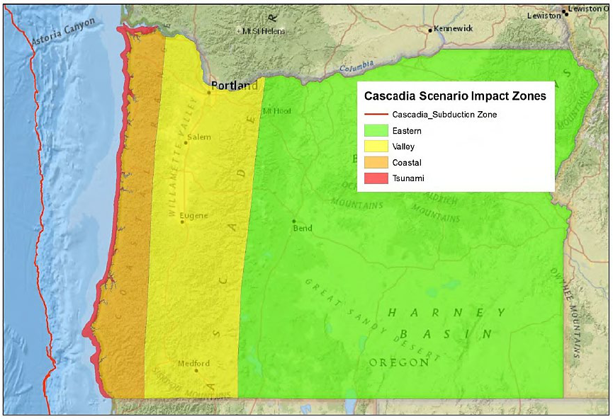
Google search intensity spikes are also in line with Crowe's (2018) findings of spikes in media
coverage following Schulz’ 2015 New Yorker article and the 2011 Tohoku earthquake and tsunami. Figure
Figure 2.
Google searches between 1/1/04 and 1/1/18 in Oregon as measured by search interest relative to the highest point
on the chart for the given region and time range. (a) For terms “Oregon earthquake”, “Cascadia subduction zone”, and
“Earthquake prediction”. (b) For terms “Oregon earthquake” and “Oregon tsunami”. The term “Oregon tsunami” is omitted
from (a) due to an order of magnitude spike in search intensity for “Oregon tsunami” during the Tohoku event relative to the
other three terms over the time range.
12
2(a) graphs the Google searches in Oregon for the terms “Oregon earthquake”, “Cascadia subduction zone”,
and “Earthquake prediction” between 2004 and 2017. Search popularity is measured as a percentage of
search interest relative to the highest point on the chart for Oregon web users (searches originating from
Oregon addresses) between 2004 and 2017 (Google Trends, n.d.). The number of searches peaked in July
2015 reflecting the viral popularity of the New Yorker article. The Tohoku earthquake and tsunami in
March 2011 represents the second highest peak in searches and was 75% as popular as the New Yorker
article. However, the search intensity for “Oregon earthquake” at its peak after the 2015 New Yorker article
is only 40% of the search intensity for “Oregon tsunami” at its peak during the 2011 Tohoku event (see
Figure 2(b)).
Combined, the increase in internet searches for information on an Oregon earthquake/tsunami and
media coverage on the CSZ immediately after these two events suggests that they acted as information
shocks to Oregon residents. The Tohoku 2011 earthquake and tsunami could have increased Oregonians’
information levels about the Cascadia event due to its similarity to the predicted Cascadia event and the
fact that its impacts were felt on the Oregon coast. The 2015 New Yorker article also likely impacted
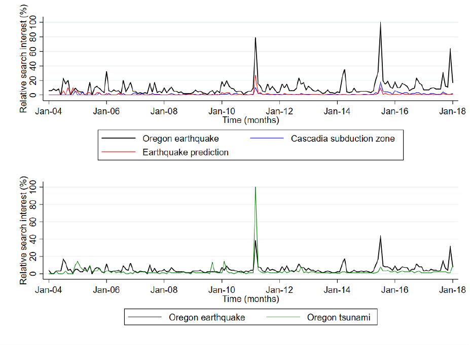
Figure 3.
Tsunami blue line signage in (a) Newport, OR (courtesy of Mike Eastman) and (b) Seaside, OR (courtesy of Anne
McBride).
13
Oregonians’ information levels and risk perceptions about the Cascadia event through its viral status and
detailed explanation and illustration of the objective risk.
Oregon has implemented several policies designed to make the public more aware of and prepared
for the Cascadia earthquake and tsunami. The Tsunami Blue Line project launched in February 2016 and
provided communities along the Oregon coast with funds and materials to install thermoplastic blue lines
and signs marking the entrance to the tsunami evacuation zone (Office of Emergency Management, 2016).
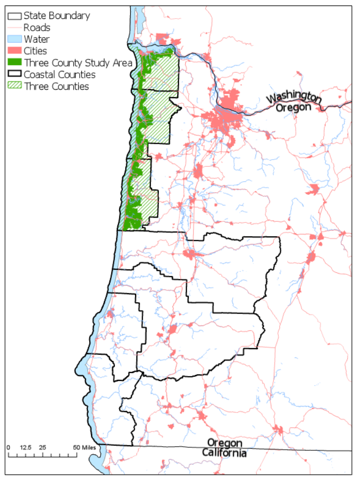
Figure 4.
GIS data for three county study area (green hatching) and the seven coastal counties (black border). Coastal counties
from north to south (unlabeled): Clatsop, Tillamook, Lincoln, Lane, Douglas, Coos, and Curry. The study area for the first
analysis (solid green) is defined to be within 1 mile of the tsunami inundation zone given by the 1995 SB 379 line.

14
The blue lines and “Leaving Tsunami Zone” signs were installed on the 2013 XXL tsunami inundation and
evacuation line at various times since 2016 through the present day. Most blue lines are approximately 12”
wide and have “Leaving Tsunami Zone” signs next to them, as seen in Figure 3(a), though some only have
the “Leaving Tsunami Zone” sign without an accompanying blue line, as seen in Figure 3(b). Thus, the
blue lines present distinct visual markers of entry/exit into the tsunami inundation and evacuation zone. The
coastal communities that had blue lines installed were Bay City, Cannon Beach, Coos Bay, Florence, Gold
Beach, Lincoln City, Manzanita/Nehalem, Newport, Reedsport, Seaside, and Yachats as well as some
unincorporated areas of Lincoln County. Each of these communities managed the installation of their own
blue lines except for unincorporated communities whose blue lines were installed by their county’s public
works department. Most of the time the blue lines and signs were installed on roads on or near the 2013
XXL tsunami line though at times the community’s input changed the location of the blue line. In addition
to a statewide press release (Office of Emergency Management, 2016) and flyers announcing the new blue
lines, several community news agencies also reported on their local blue lines following installation
(Fontaine, 2016; Kustura, 2016; Sheeler, 2018).
The first analysis in this paper focuses on the three northernmost counties of Clatsop, Tillamook,
and Lincoln because the North Oregon coast is expected to experience the most concentrated tsunami
exposure (OSSPAC, 2013).
3
Since the Tohoku earthquake/tsunami and New Yorker article are both “pure”
or “distant” information shocks, I chose to focus on the region of Oregon that is likely to be the most
sensitive to such shocks. The northern coast counties have the highest percentages of tsunami-prone land
that is zoned as urban (Wood, 2007). While 95% of the land in Oregon’s tsunami inundation zone is
classified as undeveloped, 48% of Clatsop County’s tsunami zone, 34% of Lincoln County’s tsunami zone,
and 21% of Tillamook County’s tsunami zone are zoned as urban (Wood, 2007). The northern coast cities
contain the highest number of public venues and dependent-population facilities like schools and hospitals
in the tsunami inundation zone. These cities also have the highest percentages of their employees in the
tsunami inundation zone (Wood, 2007). In 2018, the population of these counties was: 39,200 in Clatsop,
26,395 in Tillamook, and 48,210 in Lincoln (Secretary of State, n.d.-b). All three of these counties are rural
with the largest city – Newport, the county seat of Lincoln County – having a population of 10,125 in 2018
(Secretary of State, n.d.-a). Population and housing are concentrated primarily in the small incorporated
and unincorporated coastal towns of these counties. Clatsop County has five incorporated towns, Tillamook
County has seven, and Lincoln County has six. As of 2007, approximately 36% of residents in the tsunami
3
So as to measure only the “pure” information effect due to the Tohoku earthquake and tsunami and not the effect of damages
from the tsunami, Curry County (the southernmost county in Oregon) was intentionally excluded from the potential study area
because the port of Bookings experienced much higher damage than any other coastal community in Oregon. With this limitation,
the costs to the Oregon coast are then primarily the indirect cleanup costs of debris from Japan and not direct infrastructure damage.
According to local newspapers, the majority of damage occurred in southern Oregon and northern California (Jung, 2011; Tobias,
2012).
15
inundation zone lived in rural, unincorporated areas of the seven coastal counties, primarily in the
unincorporated towns of the three northern counties (Wood, 2007).
Oregon’s Office of Economic Analysis (OEA) groups these three counties together as a regional
economy. It is reasonable to consider these counties as a single housing market given their separation from
Oregon’s population centers in the Willamette Valley, their connection via HWY 101, and their similar
economies and industries. These three counties span approximately 150 miles in the north-south direction.
While it is unlikely that someone would commute over three hours from Yachats (the southernmost town)
to Astoria (the northernmost town) for work, it is plausible that people would commute half that distance.
Figure 4 shows a map of the three northern counties (green hatching) and the boundaries of the seven coastal
counties (black). The map also illustrates the clustering of and connections between population centers on
the coast, the lack of population along the Oregon Coast Range, and the separation from the urban centers
in the adjacent Willamette Valley counties.
The second and third analyses have more narrowly defined sample spaces that contain a limited
number of treated observations, necessitating an expansion to include housing data from all seven coastal
counties. For example, only eleven coastal communities received blue lines and, of these, some
communities (e.g., Cannon Beach) received as few as three blue lines. These blue lines were installed at
times between 2016 and 2019, which results in a short post-installation time range and therefore few
property sales after installation for the DID model in the third analysis. This extension assumes that the
entire Oregon Coast can be treated as a single housing market, as in Dundas and Lewis (2020). Under this
assumption, the three northern coast counties comprise a sub-market of this larger housing market.
4 Data
Multiple data sources including property sales data, tsunami inundation maps, Census block group data,
and other GIS data are used for these analyses. Property sales data was aggregated from tax assessor records
in Zillow’s ZTRAX database and spans residential, agricultural, and commercial sales from 1995 through
2018 (Zillow, 2020). These data were cleaned to remove all non-residential transactions and transactions
missing key structural variables (age, etc.). In each year, transactions with prices in the bottom one percent
were removed because they may reflect non-arms-length transfers, e.g., intra-family transfers. Transactions
in the top one percent in each year were also removed. Houses that sold more than five times between 2009
and 2018 were dropped because of potential unobservables driving their frequent resale. Potential multi-
family dwellings – properties with more than eight bedrooms or six bathrooms – were dropped from the
sample. Finally, transactions that took place less than one year since the previous sale were removed since
they often reflected either the same transaction recorded at multiple points through the sale process or a
house purchased to be flipped and re-sold. The Zillow ZTRAX data does not have reliable second home

16
indicators, however, so identifying second home ownership is not possible at this time.
4
Following this
cleaning, the remaining transactions contain only arms-length, single-family residential sales that reflect
the valuations of potential homeowners. Some of the key structural covariates from the Zillow data include
the effective age of the house (2018 – remodel year), indoor square footage, total acreage, number of
bedrooms, number of bathrooms, and whether the house has a garage.
Neighborhood and location amenity data are collected from several state and federal sources. The
majority of the data comes from the Emergency Preparedness Data Collection, the public version of a
dataset compiled by Oregon’s Preparedness Framework Implementation Team (Prep-FIT) for the Oregon
Incident Response Information System (OR-IRIS). This dataset is a collection of existing and purpose-built
GIS datasets combined to help understand the setting of a potential emergency response incident
(Preparedness Framework Implementation Team (Prep-FIT), n.d.). Sources of the OR-IRIS data include
state agencies such as the Oregon Department of Transportation (ODOT) and federal agencies such as
USGS. This data includes location information for airports, fire stations, hospitals, wastewater treatment
plants, beach access points, highways and roads, railroads, rivers and other waterbodies, the ocean
shoreline, and cities. Distance to the nearest central business district is measured as the distance to the center
of the nearest town (incorporated or unincorporated). Coastal towns are small and likely have only one
central business district. Distances to the nearest hospital, law enforcement station, fire station, and
wastewater treatment plant were included since proximity to one of these facilities may serve as a proxy
for a “safety” amenity.
Location information on state and federal protected areas (public lands) primarily came from the
USGS Protected Areas Database of the United States (PAD-US). Federal public lands were trimmed to
include conservation areas, national forests, national historic sites, national monuments, national parks,
national recreation areas, national wildlife refuges, wilderness areas, and recreation or resource
management areas. State public lands were trimmed to include only state forests, state parks, and wildlife
management areas. Elevation data was collected in 10m-by-10m pixels from the Oregon Department of
Geology and Mineral Industries (DOGAMI). GIS software was used to calculate the elevation of each
property and the distance from each property to the nearest location amenity.
5
For oceanfront properties,
4
Second homes and vacation rentals constitute a large share of housing in the northern counties due to the dominance of the tourism
sector on the Oregon coast. According to the 2019 Clatsop County Housing Strategies Report (Appendix A, 2019) the estimated
vacancy rate of ownership housing is very high, especially in beachside communities. They also find that in several beachside
communities short-term rentals have outpaced the addition of new units; an estimated 58% of new houses built in the county since
2010 are used as short-term rentals (Clatsop County Housing Strategies Report, Appendix A, 2019). Second homeowners who do
not live on the Oregon coast and directly face the risk of a Cascadia tsunami may have different risk perceptions and preferences
than permanent residents of the Oregon coast. Accounting for second home ownership is therefore important for accurately
estimating residents’ risk perceptions.
5
All distances are Euclidian. Euclidian distances may underestimate true distances in these rural counties. Also, Euclidian and
travel distances may capture different amenities. For example, I would expect that as travel distance to the nearest beach access

17
additional data on shoreline armoring and armoring eligibility is included. Shoreline armoring is a private
option to protect oceanfront properties from erosion and storm surges by installing hardened shoreline
protection structures.
6
Armoring eligibility and the existence of shoreline protective structures represent
safety amenities for oceanfront properties. Oceanfront parcels were identified using the Oregon Department
of Land Conservation & Development’s inventory of oceanfront parcels and their armoring eligibility.
Several studies have used changes in the number of insurance policies following a disaster event
as a measure of changing subjective perceptions about the expectation of a future disaster (Atreya et al.,
2013; Gallagher, 2014). This study omits insurance information primarily due to a lack of parcel-level
earthquake and flood insurance data.
7
Finer-scale fixed effects, however, should be able to capture some of
the unobservable heterogeneity due in part to earthquake insurance uptake differences between
neighborhoods. 2010 Census information was collected at the Census block group level to be used for these
neighborhood-level spatial fixed effects. Block groups generally contain between 600 and 3,000 people,
with an optimum size of 1,500 people. The block group is the smallest geographical unit above the block
level that is uniquely identified and therefore represents the smallest neighborhood unit data available.
Earthquake insurance, however, only covers damage from strong shaking but not water damage
from a tsunami (OSSPAC, 2018). Tsunami damage is typically covered by flood insurance (OSSPAC,
2018). FEMA’s National Flood Insurance Program (NFIP) requires the purchase of flood insurance for
mortgages in the 100-year floodplain – also known as Special Flood Hazard Areas (SFHA) – that are
managed by federally regulated lenders. Mortgage lenders must also inform homebuyers if the property is
located in an SFHA. On the Oregon coast, the SFHA floodplain line is similar but not identical to the
tsunami inundation lines (OSSPAC, 2018). For example, for the first analysis, only 3% of properties outside
the SB 379 tsunami inundation zone are inside a SFHA; however, 36% of properties inside the SB 379
inundation zone are also inside a SFHA (Table 1). These homes in both the tsunami inundation zone and
in the SFHA likely have flood insurance. Therefore, even without fine-scale flood insurance policy data, it
may be possible to use presence in a SFHA to roughly proxy for flood insurance ownership inside the
tsunami inundation zone. This SFHA indicator will underestimate the amount of flood insurance policies
point increases, property values decrease since beach access is an amenity. However, Euclidian distance to a beach access point
may primarily capture the visual disamenity of congestion at popular beach access points.
6
Oregon’s Statewide Planning Goal 18 designates which parcels are eligible to install shoreline armoring (Department of Land
Conservation & Development, n.d., p. 18). To limit shoreline armoring and resulting beach erosion and loss of beach access Goal
18 limits shoreline armoring to parcels where development existed prior to 1977.
7
Most homeowner insurance policies in Oregon do not cover earthquake damage though many homeowners insurance providers
offer standalone earthquake coverage and earthquake insurance is widely available through the state of Oregon (Division of
Financial Regulation, n.d.). As of 2017 approximately 14.8% of Oregonians with residential homeowners insurance also have
earthquake insurance (Cheng, 2018). This is comparable to other Pacific Coast states with high earthquake risks, e.g., Washington’s
uptake rate of 11.3% and California’s uptake rate of 15.1%. Earthquake insurance data is only available at the county level and the
variation in insurance uptake between the coastal counties is too low for the county-level information to be useful.

18
because, while most homes inside the SFHA have flood insurance, some homes outside the SFHA may also
have flood insurance but will not be picked up by the SFHA indicator.
For the first analysis, the sample space of transactions was limited to those properties within 1 mile
of the original tsunami inundation zone (SB 379). This removes non-coastal properties on the eastern side
of the county from the sample. Non-coastal properties likely have different amenity sets than coastal
properties so their removal from the sample better controls for omitted neighborhood and location
amenities. A distance of 1 mile from the SB 379 line captures all of the towns in the three counties and does
not extend into large rural or forest parcels on the eastern sides of the counties.
8
The temporal extent of the
first analysis is 2009 to 2017 so that each event – the 2011 earthquake and the 2015 article – is bracketed
by two years of property sales data before and after the event. The Zillow data spans the years 2009 to 2017
and contains 15,627 transactions.
9
The tsunami inundation zones that define the treatment group in the first analysis include the 1995
SB 379 line and the largest of the 2013 TIM scenarios (XXL). Table 1 compares the descriptive statistics
of houses inside and outside the 1995 SB 379 tsunami inundation zone to illustrate differences between the
treatment and control groups for the sample used in the first analysis. Approximately 27% of the
transactions between 2009 and 2017 were inside the SB 379 inundation zone. The houses inside and outside
the SB 379 zone are similar in terms of effective age, total acreage, number of bedrooms and bathrooms,
and whether they have a fireplace or external structures (e.g., garage, patio, fencing). Houses inside the
inundation zone on average sell for $16,000 more which likely reflects the shorter distances to likely
amenities such as the ocean, rivers, public lands, and schools and the greater distances to likely disamenities
such as highways. Houses outside of the inundation zone have larger indoor square footage and total acreage
which may be due to the higher density of houses inside the inundation zone. Approximately 99% of the
houses inside the SB 379 inundation zone are also in the 2013 XXL scenario inundation zone. The XXL
scenario of the 2013 TIM series was in use for official tsunami evacuation maps during the 2015 New
Yorker article. Approximately 49% of the transactions between 2009 and 2017 were in this inundation
zone.
10
The change in tsunami inundation and evacuation maps between the two events of interest presents
a model specification problem that is addressed in section 5.1. See Appendix A.2 for figure comparisons of
the 2013 TIM and 1995 SB 379 tsunami inundation scenarios for the city of Tillamook.
8
Distance to the SB 379 tsunami inundation zone was chosen instead of distance to the shoreline only because the ocean shoreline
data does not extend into the Columbia River on the northern boundary of the three-county area and the SB 379 data does extend
into the Columbia.
9
Table A1 in Appendix A.3 presents summary statistics for the sample used in the first analysis, i.e., for 2009-2017 property sales
that occur within 1 mile of the 1995 SB 379 line in the three northern counties.
10
See Table A1 in Appendix A.3.

19
Table 1. Variable Definitions and Descriptive Statistics, by SB 379, First Analysis Sample, 2009-2017
Outside SB 379 zone
Inside SB 379 zone
Mean
Std dev
Mean
Std dev
Std diff in
means
Event
Sold after 2011 Tohoku EQ
(tohoku=1)
0.81
(0.39)
0.81
(0.39)
-
Sold after 2015 article (article=1)
0.33
(0.47)
0.32
(0.47)
-
Treatment
Inside 1995 SB 379 tsunami zone
(sb379=1)
0
(0)
1
(0)
-
Inside 2013 XXL tsunami zone
(xxl2013=1)
0.31
(0.46)
0.99
(0.09)
-
Inside 2013 XL tsunami zone
(xl2013=1)
0.28
(0.45)
0.99
(0.10)
-
Inside 2013 L tsunami zone (l2013=1)
0.12
(0.33)
0.96
(0.20)
-
Inside 2013 M tsunami zone
(m2013=1)
0.04
(0.20)
0.82
(0.38)
-
Inside 2013 SM tsunami zone
(sm2013=1)
0.01
(0.09)
0.47
(0.50)
-
Structural
Sale price (2019 constant dollars)
306,745.77
(163,480.12)
323,071.60
(186,908.93)
-0.09
Bedrooms
2.89
(0.92)
2.68
(0.93)
0.23
Bathrooms
2.06
(0.78)
1.90
(0.75)
0.22
Indoor square footage
1,744.24
(715.21)
1,505.16
(645.45)
0.35
Total acreage (equal to indoor area if
apartment)
0.42
(2.13)
0.33
(2.28)
0.04
Effective age of property (2018 -
remodel year)
35.97
(25.54)
36.43
(24.46)
-0.02
Heating (=1)
0.95
(0.22)
0.91
(0.29)
0.17
Fireplace (=1)
0.66
(0.47)
0.61
(0.49)
0.09
Garage (=1)
0.77
(0.42)
0.69
(0.46)
0.18
Carport (=1)
0.04
(0.20)
0.03
(0.18)
0.04
Deck (=1)
0.11
(0.31)
0.16
(0.36)
-0.14
Patio (=1)
0.17
(0.38)
0.20
(0.40)
-0.07
Fencing (=1)
0.14
(0.35)
0.18
(0.38)
-0.10
Goal 18 eligible (=1)
0.02
(0.13)
0.10
(0.30)
-0.35
Has shoreline armoring (=1)
0.00
(0.05)
0.04
(0.20)
-0.28
Location
Special Flood Hazard Area (SFHA)
(=1)
0.03
(0.16)
0.36
(0.48)
-0.94
Elevation (ft)
97.42
(70.54)
20.95
(11.02)
1.51
Slope (angular degrees of slope)
2.72
(4.82)
1.74
(2.38)
0.26

20
The last column of Table 1 presents the standardized difference in means for the structural and
location covariates. Several key explanatory variables such as elevation (1.51) and distance to the ocean
shoreline (0.55) have large absolute standardized differences (in parentheses). Some researchers have
suggested that an absolute standardized difference of 0.25 or more indicates that covariates are imbalanced
between groups (Stuart, 2010). This suggests that the treated and control groups are considerably
imbalanced and that covariate balancing, e.g., matching or weighting, may be useful or necessary for
identification.
For the second analysis, the sample space of transactions is limited to those properties that were
outside of the original 1995 SB 379 tsunami evacuation zone. The 2013 update of tsunami inundation and
evacuation maps represents an exogenous risk signal to houses that were outside of the original 1995 SB
379 inundation zone but with the hazard planning change found themselves inside one of the new 2013
inundation zones. As such, each of the five 2013 tsunami inundation zones is used as the treatment boundary
Distance to nearest beach access point
(ft)
4,348.03
(6,943.63)
2,075.03
(4,633.56)
0.39
Distance to ocean shoreline (ft)
16,402.69
(23,311.22)
5,926.15
(13,706.17)
0.55
Oceanfront (=1)
0.03
(0.16)
0.11
(0.32)
-0.35
Distance to nearest water body (lake,
pond, bay) (ft)
6,977.92
(7,673.00)
6,437.03
(9,694.99)
0.06
Distance to nearest river (ft)
8,155.13
(8,038.36)
4,987.01
(7,363.52)
0.41
Distance to nearest state park or public
land (ft)
25,889.50
(26,449.02)
21,853.60
(24,369.87)
0.16
Distance to nearest national park or
public land (ft)
17,547.64
(16,187.60)
20,618.42
(18,961.51)
-0.17
Distance to nearest highway or
interstate (ft)
2,735.67
(4,070.97)
4,346.39
(6,942.60)
-0.28
Distance to nearest major road (ft)
3,173.23
(5,045.23)
5,383.81
(8,321.11)
-0.32
Distance to nearest railroad (ft)
68,837.11
(60,557.73)
83,561.70
(51,105.73)
-0.26
Distance to nearest airport (ft)
32,312.90
(19,089.39)
26,215.34
(19,586.41)
0.32
Distance to nearest k-12 school (ft)
14,668.42
(15,629.87)
12,327.99
(10,823.89)
0.17
Distance to nearest central business
district (city) (ft)
11,027.20
(10,671.49)
9,171.75
(8,882.89)
0.19
Distance to nearest wastewater
treatment plant (ft)
15,651.49
(11,137.14)
11,604.52
(9,447.23)
0.39
Distance to nearest fire station (ft)
5,992.65
(4,597.47)
6,141.79
(5,116.56)
-0.03
Distance to nearest law enforcement
station (ft)
30,593.44
(35,657.69)
34,384.59
(44,793.06)
-0.09
Distance to nearest hospital (ft)
45,555.14
(42,443.18)
54,716.99
(45,225.25)
-0.21
Observations
11,467
4,160

21
for a separate sample where the sample is restricted to a narrow band of properties within 1 mile of the
treatment boundary given by the XXL, XL, L, M, or SM inundation line. Table 2 compares the samples of
the resulting five different sample spaces and lists the number of transactions inside and outside the given
inundation zone for each sample. This table illustrates the data limitations of this analysis even after
extending the sample space to all seven coastal counties, as can be seen by the small number of treated
observations (81) available for the SM inundation line treatment boundary sample. The time range for this
analysis is from 2011 to 2015 so that the 2013 evacuation map change is bracketed by two years of property
sales data before and after the event.
11
The third analysis restricts the sample space to a small neighborhood of properties around newly
installed blue lines and the 2013 XXL inundation line. The preferred model restricts treated observations
to be within 1000’ of the blue line and control observations to be within 2500’. The temporal extent of the
sample is 2014 and 2018 so that each blue line has at most two years of property sales before and after its
installation since the blue lines were installed at different times between 2016 and 2019.
12
Table A4 in
Appendix A.3 compares the descriptive statistics of houses inside and outside the blue line neighborhood
given by a 1000’ radius to illustrate differences between the treatment and control groups for the sample
used in the preferred model. This table shows that the standardized differences in means for this sample
space are small in comparison to the sample spaces of the first and second analyses. This suggests that the
11
Table A2 in Appendix A.3 presents summary statistics for the sample used in Model 1 of the second analysis, i.e., for 2011-2015
property sales that are outside the 1995 SB 379 line and are within 1 mile of the 2013 XXL line in the seven coastal counties. This
is the largest sample space in the second analysis and encompasses the other four sample spaces. Table A3 in Appendix A.3
compares the descriptive statistics of houses inside and outside the 2013 SM tsunami inundation zone to illustrate differences
between the treatment and control groups for the sample used in Model 5. This is the smallest sample space and has the largest
standardized differences in means. Descriptive statistics for the remaining samples used in this analysis are not presented here but
are available upon request.
12
For blue lines installed in 2018 less than one year of property sales is available post-installation. For blue lines installed in 2019,
there are no post-installation property sales. This is due to a lack of updates to ZTRAX housing transactions after 2018 for most
Oregon counties (as of June 2021).
Table 2. Second Analysis Samples, 2011-2015
Sample
Model
Total
observations
Outside inundation
zone
Inside inundation
zone
Within 1 mile of the XXL
inundation zone
1
8,010
5,855
2,155
Within 1 mile of the XL inundation
zone
2
7,790
5,829
1,961
Within 1 mile of the L inundation
zone
3
6,593
5,698
895
Within 1 mile of the M inundation
zone
4
5,842
5,527
315
Within 1 mile of the SM inundation
zone
5
5,429
5,348
81
22
narrow sample space definition successfully restricts neighborhoods to be more homogenous and thus may
help deal with time-invariant and time-varying unobservables that may be correlated with either proximity
to the blue lines or the 2013 XXL line.
A database of blue line locations and installation dates does not exist at the state or county levels.
Thus, information about when and where the blue lines were installed was gathered by contacting individual
city and county emergency managers, public works departments, and planning departments along the
Oregon coast. Emails and phone conversations were used to compile a list of approximate blue line
locations and installation times. Some locations were given as being in the vicinity of street intersections
or nearby landmarks so I approximate the location of the blue line based on the location of the 2013 XXL
tsunami inundation line and this firsthand information. Timing information was provided as the month and
year of installation. However, sometimes no timing information other than the year of installation was
available. This ambiguity of installation dates further reduces the post-installation time range for the DID
and DDD models. Timing and location information is currently incomplete for several towns that are known
to have blue lines installed, usually due to multiple blue line installation periods or uncertainty about
whether some blue lines were installed. Due to the potential non-randomness of this missing data, these
towns were not included in the dataset analyzed in this paper.
5 Methodology
5.1 First analysis: 2011 Tohoku earthquake and tsunami and 2015 New Yorker article
In the first analysis, I use two exogenous information shocks to distinguish between the effect of coastal
amenities and the increased subjective risk of tsunami inundation. I use a difference-in-differences (DID)
model to difference out time-invariant omitted variables and contemporaneous effects such as
macroeconomic shocks. There is a complication with defining the treatment group (inside the tsunami
inundation zone) and control group (outside of the inundation zone) because the DOGAMI tsunami
inundation maps changed in 2013 from the SB 379 line to the new TIM Plate 1 series. This motivates three
model specifications. For the first specification (Model I), I consider only the Tohoku earthquake event and
the 1995 SB 379 tsunami line as the boundary between the treatment and control groups. The time range
for this specification is from 2009 to 2013 (before the DOGAMI tsunami inundation maps change). The
model specification is:
(
)
=
+
379
+
+
379
+
+
+
,
(
1
)
where
is the sale price (in constant 2019 dollars) of house with structural and location
characteristics in Census block group at time . The log transformation of
was chosen as the

23
dependent variable in all models because taking the log of narrows its range and can make estimates
less sensitive to extreme values. The treatment variable 379
indicates whether the house is in the tsunami
inundation zone given by the 1995 SB 379 scenario. The event variable
indicates that the sale
happened after 3/11/2011 (the post-Tohoku period).
13
The parameter of interest is
, the marginal effect
of the Tohoku 2011 earthquake and tsunami on property values inside the tsunami inundation zone given
by the 1995 SB 379 scenario. The structural characteristics in
include quadratic terms for the non-binary
variables to better account for their expected diminishing effect on property prices (e.g., Atreya et al., 2013;
Bin & Landry, 2013). I also follow previous hedonic studies and take log transformations of the distance
variables (originally in feet) in
to abstract from unit issues (Atreya et al., 2013; Bin & Landry, 2013).
The temporal fixed effects
were included to capture any seasonal (90-day) heterogeneity or
shocks that affect all property sales. The Census block group spatial fixed effects
are interacted
with the annual fixed effects
in
to capture how these neighborhoods are changing
over time. These spatial-temporal fixed effects soak up annual changes at the neighborhood level such as
storm surges and allow neighborhoods to flexibly differ in their recoveries from the subprime mortgage
crisis and Great Recession.
14
Model II considers the New Yorker event and the largest scenario (XXL) of the new 2013 tsunami
zones as the boundary between treatment and control groups. The time range for this specification is 2013
– 2017. While the SB 379 is most comparable to the M and L scenarios by area, the XXL scenario was
chosen as the treatment for Model II because it is the most extreme scenario. I expect that households
willing to pay a risk premium to avoid tsunami inundation will likely choose to locate outside the entire
region of potential tsunami inundation. The XXL scenario is also the scenario used by DOGAMI to create
their tsunami evacuation maps, making it the most salient scenario for the public at large. The model
specification for Model II is:
(
)
=
+
2013
+
+
2013
+
+
+
(
2
)
The treatment variable 2013
indicates whether the house is in the tsunami inundation zone given by
the 2013 XXL scenario. The event variable
indicates the sale happened after 7/20/2015 (the post-
13
The
event variable is defined as between 3/11/2011 and 7/20/2015 (the post-Tohoku period and pre-New Yorker article
period). Since the time range for Model I is from 2009 to 2013, the
variable equals 1 for all sales during this time that
occur after the Tohoku earthquake and tsunami on 3/11/2011. The
variable definition is discussed further in the Model
III specification section.
14
The appropriate scale at which Great Recession recovery is capitalized may be at shorter time scales, i.e., at the
scale. This fixed effect is tested as a robustness check.
24
New Yorker article period). The parameter of interest is
, the marginal effect of the 2015 New Yorker
article on property values inside the tsunami inundation zone given by the 2013 XXL scenario.
Model III incorporates the New Yorker article event into Model I and keeps the 1995 SB 379
tsunami line as the treatment boundary. Since the 2013 tsunami inundation maps are only two years old and
the 1995 map had been in circulation for 20 years by the New Yorker article’s publication, there could be
a lag in the public’s knowledge and acceptance of the new tsunami boundaries. This specification assumes
an information lag and that homebuyers place more importance on the long-standing SB 379 line when
choosing where to locate. The time range for this specification is 2009 to 2017. The DID model
specification for Model III is:
(
)
=
+
379
+
+
+
379
+
379
+
+
+
(
3
)
The implicit assumption in the definition of the
variable here is that the impact of the 2011 Tohoku
earthquake/tsunami on property values decreases over time and disappears by the New Yorker article in
2015. This assumption follows previous findings that risk premiums decay over time and may disappear if
additional disaster events do not occur (Atreya et al., 2013; Bin & Landry, 2013; Hansen et al., 2006;
Kousky, 2010; McCluskey & Rausser, 2001; McCoy & Walsh, 2018). The parameters of interest are
and
, the marginal effects of the 2011 earthquake/tsunami and 2015 article on property values inside the
tsunami inundation zone given by the 1995 SB 379 scenario.
Consistent estimation of these treatment effects requires the parallel trends assumption. The parallel
trends assumption requires that absent the two information shocks, the difference in unobserved property
price drivers between properties inside the tsunami inundation zone and outside the tsunami inundation
zone would have remained constant. I assess the validity of this assumption in Figure 5, which plots residual
housing prices inside and outside of the treatment inundation line – SB 379 or 2013 XXL, depending on
the model – for the three northern counties. To account for observable differences across houses, I first
regress log sale prices on structural attributes, location covariates, and fixed effects for quarter and Census
block group by year. I then aggregate the residuals to the group (treated or control) and month level and
plot these residuals over time using local polynomial regressions. Figure 5(a) plots the housing price trends
inside and outside of the 1995 SB 379 tsunami inundation zone for Model I’s time range – March 2011 to
March 2013. Adjusted prices of the treated group before the 2011 Tohoku earthquake and tsunami exhibit
a similar trend as those of the control group. Following the 2011 Tohoku event, residual prices for the
treated group initially drop but then recover to nearly pre-treatment levels by 2013. Figure 5(b) plots the
housing price trends inside and outside of the 2013 XXL tsunami inundation zone for Model II’s time range
– July 2013 to July 2017. Before the 2015 New Yorker article, the treated group exhibits a similar trend as
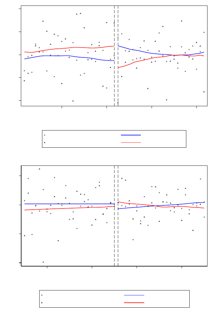
25
the control group. However, residual prices for the treated group appear to increase following the 2015
article event, a counterintuitive result.
Following the estimation of the DID regressions, I test whether the resulting risk discounts decay
over time. However, the literature on how to measure these decay effects is not standardized and a variety
(a)
(b)
Figure 5.
Housing price trends inside and outside of the treatment inundation line – SB 379 or 2013 XXL – for the three
counties. Plot of residual (log) sale prices net of structural attributes, location covariates, and fixed effects aggregated by month
with local polynomial trend lines. (a) For Model I’s time range. (b) For Model II’s time range.
2011 Tohoku EQ
-.2 -.1
0 .1 .2
Residual log sale prices
2010
2011
2012
2013
Year
Control (outside SB 379) Control trend
Treatment (inside SB 379) Treatment trend
2015 Article
-.2 -.1 0 .1
Residual log sale prices
2014
2015
2016
2017
Year
Control (outside 2013 XXL) Control trend
Treatment (inside 2013 XXL) Treatment trend

26
of methods exist that attempt to measure the decay effect. I use a method similar to the one used by Bin and
Landry (2013). This method uses only data after the event and regresses log sale prices on the treatment
variable, a count of months between the event and the month of sale
(
)
, and the interaction
between the two. For example, the specification for the SB 379 tsunami inundation zone is:
(
)
=
+
379
+
+
379
(
)
+
+
+
(
4
)
Different specifications are used for
(
)
transformation including linear, log, square root, and
ratio specifications, i.e.,
, ln
(
)
,
,
. The parameter of
interest is
, the coefficient on the interaction between the
(
)
transformation and the
treatment variable. A positive and statistically significant coefficient suggests that the risk premium is
decaying over time (Bin & Landry, 2013).
An important identification concern is the covariate imbalance found for several key explanatory
variables. Estimating average treatment effects using ordinary linear regression methods becomes more
challenging when there is considerable imbalance in covariates between the treatment and control groups.
Matching and weighting methods were developed to estimate average treatment effects under weaker
assumptions by avoiding distributional and functional form assumptions (Imbens, 2004). Matching
methods can also be used to preprocess data to improve causal inference (Ho et al., 2007). Methods that
combine matching (to preprocess the data) and regressions are more robust against misspecification of the
regression function than regressions alone (Imbens, 2004).
To improve covariate balance and potentially increase robustness against model misspecification I
pre-process the data using four matching methods – nearest neighbor propensity score matching (PSM),
nearest neighbor Mahalanobis (NNM) distance matching, coarsened exact matching (CEM), and entropy
balancing (EB) as robustness checks. Although they are popular matching methods, both PSM and NNM
are also members of a class of methods known as “Equal Percent Bias Reducing” (EPBR), which have been
shown to not guarantee imbalance reduction for any given data set and to rely on a set of strict and
unverifiable assumptions about the data generating process (Iacus et al., 2011, 2012). Iacus et al. (2011)
introduce a new class of matching methods that have many attractive properties and require fewer
assumptions. In one of these methods, CEM, each variable is coarsened so that similar values are grouped
into a stratum and assigned the same value. Then, an exact matching algorithm is applied to the coarsened
data so that control units within each stratum are weighted to equal the number of treated units in that
stratum. Strata without at least one treated and one control unit are discarded. The remaining units with
their original uncoarsened variable values form the matched data set. Entropy balancing is a weighting
method (Hainmueller, 2012) that, like CEM, specifies constraints on covariate balance before the

27
preprocessing adjustment. Entropy balancing is designed to improve balance on all covariate moments by
directly incorporating covariate balance into the weight function applied to the data. This method directly
adjusts the unit weights of the control group to match the moments of the treatment group while also keeping
the control weights as close as possible to the base weights. Unlike CEM, entropy balancing does not
discard treated units.
While there are various guidelines for selecting variables for matching, there is a consensus that
only those covariates anticipated to influence both treatment and the outcome variable should be included
(Brown & Atal, 2019; Caliendo & Kopeinig, 2008). The explanatory variables that likely influence
treatment (tsunami inundation zone) assignment are elevation and distance to the ocean. I also match on
the event(s) of interest to distinguish potential matches between pre and post event.
15
To further anchor the
matched observations in time, I match on the year the property was sold (Muehlenbachs et al., 2015). For
the PSM and NNM matching methods, I use a k-nearest neighbor matching (k=1) algorithm with
replacement. Matching with replacement is recommended when there are few comparable control
observations, as here (Caliendo & Kopeinig, 2008). For the CEM method, I use the default Sturges binning
algorithm to coarsen the data. The EB method does not discard units, unlike the other three methods, and
instead generates weights to be used in the DID regressions.
16
As another robustness check, I also run a Oaxaca-Blinder regression (Blinder, 1973; Oaxaca, 1973).
The Oaxaca-Blinder regression decomposes the difference in average outcomes into a component that is
explained by group differences in the predictors and a part that remains unexplained by these differences.
This second component is called the unexplained component and can be interpreted as the average treatment
effect on the treated (ATET), much like the DID estimator (Fortin et al., 2010; Słoczyński, 2015). In the
Oaxaca-Blinder regression weights are used to generate exact covariate balance between treated and control
groups (Kline, 2011). The Oaxaca-Blinder estimator is “doubly robust” in that it is consistent if either the
model for the potential outcomes or the model for the propensity score is correct (Kline, 2011). The Oaxaca-
Blinder estimator is also easily implemented in unbalanced designs with few treated units and many controls
(Kline, 2011) and has been used previously in a coastal hedonic setting (Dundas, 2017). Practically, I
compute the two-fold decomposition using the coefficients from a pooled model over both groups (treated
and control) as the reference coefficients (Jann, 2008). The treated group is those houses inside the given
inundation zone after the event, i.e., the treated group is represented by the DID interaction term. Thus, the
Oaxaca-Blinder estimator can be computed for Models I and II but not for Model III since Model III
contains two events and therefore two treated groups.
15
NNM allows for exact matching the event variable.
16
The other three matching methods can also generate weights to be used in the DID regressions.

28
The event study design extends the standard DID by replacing the single “post event” indicator
with binary lag and lead variables that indicate whether the given observation occurred a given number of
quarters away from the event of interest. Thus, as an alternative to the DID specification, I specify event
study designs for the models with only one event of interest. Lastly, I perform four sets of falsification tests.
In the first and second sets of tests I shift the date of the 2011 Tohoku earthquake/tsunami in Models I and
III to one year before the true event and to one year after the true event, respectively, as in Atreya and
Ferreira (2015). In the third and fourth sets of tests, I follow Bakkensen et al. (2019) and randomize
treatment exposure in both the spatial (randomly assign sales to either the control or treatment group in all
three models) and temporal (randomly assign sales to either pre- or post-event in Models I and II)
dimensions.
5.2 Second analysis: 2013 change in tsunami evacuation maps
The second analysis uses residential housing sales data before and after the 2013 tsunami inundation and
evacuation map change to measure its impact on coastal Oregon property values. Since there are five 2013
inundation zones in the TIM Plate 1 map series, I need to specify five different models to capture all relevant
event and treatment combinations. Model 1 uses the XXL line as the treatment boundary, Model 2 uses the
XL line, Model 3 uses the L line, Model 4 uses the M line, and Model 5 uses the SM line. The sample is
comprised of properties outside of the 1995 SB 379 evacuation zone and restricted to a narrow 1-mile band
of properties around the treatment boundary given by the XXL, XL, L, M, or SM inundation line, depending
on the model. Thus, the control group consists of properties that are not in either (1995 or 2013) evacuation
zone and the treatment group consists of properties that were not in the 1995 SB 379 evacuation zone but
following the map change are in the XXL, XL, L, M, or SM inundation zone. The DID specification is:
(
)
=
+
2013
+
+
2013
+
+
+
,
(
5
)
where the treatment variable 2013
indicates whether the house is in the tsunami inundation and
evacuation zone given by one of the five 2013 inundation zones. The event variable
indicates
that the sale happened after the 2013 map change (10/2/2013 and later).
17
The time range for this
specification is 2011 to 2015 so that the 2013 evacuation map change is bracketed by two years of property
sales data before and after the event. The parameter of interest is
, the marginal effect of the 2013 map
change on property values outside of the original 1995 SB 379 inundation zone and inside a new 2013
17
DOGAMI released updated tsunami inundation maps by county throughout 2013. An October 2
nd
, 2013 news release by
DOGAMI states that inundation maps had been released for the entire coast, suggesting that this date could be considered as the
date of completion for the map change (DOGAMI, 2013).

29
inundation zone. This analysis uses the same temporal and spatial-temporal fixed effects as the first
analysis.
18
I assess the validity of the parallel trends assumption as in the first analysis. Figure A3 in Appendix
A.4 plots residual housing prices inside and outside of the treatment inundation line – XXL, XL, L, M, or
SM – for the seven coastal counties. The takeaway from these plots is that before the 2013 map change
only Model 1 (XXL line) and Model 5 (SM line) have treated and control groups that exhibit parallel pre-
trends. However, counterintuitively, in Model 1 the residual prices for the treated group appear to increase
following the 2013 map change. In fact, Model 5 is the only model where the residual prices for the treated
group appear to drop following the 2013 map change, as expected.
As a robustness check, I estimate a pooled model with all five 2013 tsunami inundation zones as
treatments in a single model. This model uses the sample space of Model 1 (XXL line) because it
encompasses the samples of the other four models. Similar to the first analysis, I also run Oaxaca-Blinder
regressions, specify event study designs, and perform the four sets of falsification tests for all five models.
Lastly, I test whether the risk discounts from the DID regressions decay over time using the method of Bin
and Landry (2013).
5.3 Third analysis: Tsunami Blue Line project
The third analysis measures the impact of the Tsunami Blue Line project on coastal Oregon property values
using residential housing sales data before and after the installation of the blue lines. Starting in 2016 the
Tsunami Blue Line project installed thermoplastic blue line signs on the 2013 XXL tsunami inundation and
evacuation line. Properties are differentiated by proximity to blue lines and by whether they are inside the
2013 XXL tsunami inundation and evacuation zone. The sample is restricted to a circular neighborhood of
properties around the blue lines, signifying that those properties are adjacent to a blue line. Circular
neighborhoods are the result of defining proximity to a blue line using a single distance, i.e., a distance
radius will trace out a circular neighborhood or buffer around that blue line. This also restricts the sample
to small neighborhoods around the 2013 XXL line. In practice I use two different types of distances to
define the circular treatment and control buffers: Euclidian distances, which measure the straight-line
distance between each blue line and transaction, and road network distances, which measure the shortest
path between each blue line and transaction along the road network. Figure 6 shows a taxlot map with
example treatment and control groups around a blue line (small red squares) in Manzanita, OR. The
treatment group is given by those property sales (small gray circles) inside the neighborhood around the
18
Covariate imbalance is an identification concern for several models in this analysis, e.g., Model 5 has large standardized
differences in means for several key explanatory variables (see Table A3 in Appendix A.3). Models 1 and 2 have less covariate
imbalance than Models 3 through 5. However, the number of observations for Models 3, 4, and 5 (see Table 2) is too small for the
matching methods to be able to produce useful matched samples. Thus, I forego matching or weighting for the models in this
analysis.
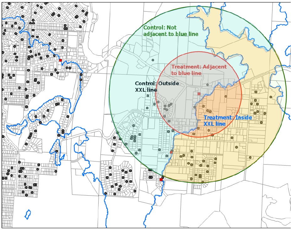
30
blue line (red circular buffer). The corresponding control group is those property sales outside of the blue
line neighborhood (red circular buffer) but inside a slightly larger neighborhood surrounding it (green
circular buffer). The 2013 XXL inundation and evacuation line (thick blue line) separates houses that are
more sensitive to the blue line treatment – houses inside the inundation zone – from those that are less
sensitive to the treatment. One identification issue is how to deal with overlapping neighborhoods for blue
lines that are in close proximity to each other. For example, figure 6 shows that the control group (green
circular buffer) encompasses a blue line in its lower left. This impacts how I define the treatment indicator.
Two new binary indicators are needed for the DID and DDD models: treatment and event. The
treatment variable indicates whether the house is in the neighborhood around the blue line, which is
complicated by the potential for multiple blue line neighborhoods to overlap a transaction. The event
Figure 6.
Taxlot map with example treatment and control groups around a blue line (small red squares) in Manzanita, OR.
The treatment group (red circular buffer labeled “Treatment: Adjacent to blue line”) and control group (green circular buffer
outside of the red circular buffer labeled “Control: Not adjacent to blue line”) represent whether property sales (small gray
circles) are adjacent to the blue line or not, respectively. The 2013 XXL inundation and evacuation line (thick blue line) separates
houses that are more sensitive to the treatment (yellow area labeled “Treatment: Inside XXL line”) from those that are less
sensitive to the treatment (green area labeled “Control: Outside XXL line”).

31
variable indicates that the sale happened after the blue line was installed, which is also complicated by the
problem of “which blue line?” To generate these indicators and deal with the overlap issue I focus on the
timing of treatment instead of on spatial controls. The key idea is that “earliest supersedes nearest.” If a
transaction lies within a given buffer distance of two different blue lines and one of the blue lines is installed
before the transaction and the other is installed after the transaction, I use the first installed blue line as the
reference point, not the nearest blue line. In case there is a tie for earliest – multiple blue lines were installed
at the same time – then the nearest blue line is chosen. To create the “treatment” variable, I consider all
possible cases of buffer overlap. The key question is how should we treat transactions that fall in one blue
line’s “treatment” buffer and another blue line’s “control” buffer? There are nine total cases that can occur
when a treatment buffer and control buffer overlap for a transaction. Appendix A.4 illustrates all nine cases
and explains how treatment and event status were defined. Essentially, if multiple blue lines fall within a
given radius (buffer distance) of the transaction in question, one blue line is chosen as the appropriate
reference point. Then, the values of the treatment and event indicators are determined by whether the
transaction is within the given radius of that blue line and whether the sale occurred after the blue line was
installed, respectively.
I test a variety of neighborhood sizes around the blue lines, i.e., the radii for the treatment and
control buffers. I run 100 models by varying the treatment buffer radius between 500’ and 3000’ and the
control buffer radius between 1000’ and 8000’.
19
Each model is defined by the treatment buffer size and
control buffer size combination that determines its sample space. Models 1 through 50 use Euclidian
distances to define the treatment and control buffers and Models 51 through 100 use road network distances.
I hypothesize that this effect will probably be highly localized so smaller buffer sizes are more likely to
show a treatment effect. The DID specification for all 100 models is:
(
)
=
+
+
+
+
+
+
,
(
6
)
where the treatment variable
indicates whether the house is in the neighborhood around the blue
line. The event variable
indicates that the sale happened after the blue line was installed.
Since the blue lines were installed at different times between 2016 and 2019, the timing of the event variable
is different between blue lines. The parameter of interest is
, the marginal effect of proximity to the blue
lines on property values.
The DDD specification adds the variable 2013
, which indicates whether the house is inside
the 2013 XXL inundation zone:
19
I test 100 models to determine the likely spatial extent of this effect. However, I do not believe that there are 100 possible valid
models for this analysis. Thus, while I do apply multiple hypothesis testing corrections, I do not apply them to all 100 models.
Section 6.3 elaborates on the 100 models tested and the hypothesis testing corrections performed.

32
(
)
=
+
+
+
2013
+
+
2013
+
2013
+
2013
+
+
+
(
7
)
The parameter of interest is
, the marginal effect of proximity to the blue lines on property values for
properties inside the 2013 XXL tsunami inundation and evacuation zone.
This analysis faces an identification challenge: variation in treatment timing. Specifically, this is a
staggered adoption design: units are treated at different times and once units are treated, they remain treated
in the following periods. The canonical DID setup has two time periods and two groups: no units are treated
in the first period and then some units become treated in the second period (the treated group) while other
units remain untreated (the control group). This model is often estimated with the standard two-way fixed
effects (TWFE) regression, as in equation (6). Several recent studies have found that under treatment effect
heterogeneity the TWFE estimator recovers a weighted average of some underlying treatment effect
parameters (Borusyak & Jaravel, 2017; de Chaisemartin & D’Haultfœuille, 2020; Goodman-Bacon, 2018;
Sun & Abraham, 2020).
20
The problem is that some of these weights can be negative, suggesting that the
TWFE estimator can be opposite in sign from the true average treatment effects. Furthermore, these weights
are sensitive to the size of each group, the timing of treatment, and the total number of time periods
(Callaway & Sant’Anna, 2020). Sun and Abraham (2020) show that the standard event study estimator
suffers from a similar problem – it is contaminated by treatment effects from other periods. Some of these
studies have proposed measures to assess these weights and how robust the TWFE estimator is to
heterogeneous treatment effects (de Chaisemartin & D’Haultfœuille, 2020; Goodman-Bacon, 2018; Sun &
Abraham, 2020). I calculate the measure proposed by de Chaisemartin and D’Haultfœuille (2020) to assess
the robustness of the TWFE estimator to heterogeneous treatment effects.
de Chaisemartin and D’Haultfœuille (2020) also propose a new DID estimator that estimates the
treatment effect in the groups that switch treatment, at the time when they switch. This estimator is valid in
staggered adoption designs and when the treatment effect is heterogeneous over time. Callaway and
Sant’Anna (2020) develop another framework for DID setups with multiple time periods and variation in
treatment timing that is valid in the presence of treatment effect heterogeneity. Their framework is based
on estimating group-time average treatment effects, which are the average treatment effect for group at
time where a “group” is defined by the time when units are first treated. The group-time average treatment
effects can be averaged into an aggregate measure: the “average effect of participating in the treatment
20
Baker et al. (2021) use simulations to show that DID estimates are unbiased in settings where there is a single treatment period,
i.e., the canonical 2x2 DID setup, even when there are dynamic treatment effects. Due to this result, I did not use the new DID
estimators that are valid in the presence of treatment effect heterogeneity in the first and second analyses.

33
experienced by all units that ever participated in the treatment” whose interpretation is like the average
treatment effect on the treated (ATET) in the TWFE DID setup. I estimate both of these new estimators
(Callaway & Sant’Anna, 2020; de Chaisemartin & D’Haultfœuille, 2020).
6 Results
6.1 First analysis: 2011 Tohoku earthquake and tsunami and 2015 New Yorker article
Table 3 reports selected estimation results of the key coefficients for Models I through III in the first
analysis.
21
The difference-in-differences (DID) coefficients are statistically significant (at the 5%
significance level) for the 2011 Tohoku earthquake and tsunami in both Models I and III. The DID estimator
for the 2015 New Yorker article is not statistically significant in either Model II or III. According to the
coefficient estimate from Model I, a property inside the SB 379 tsunami inundation zone has a risk discount
of 8.5% following the Tohoku event. The coefficient estimate from Model III implies a slightly smaller risk
21
Table A9 of Appendix A.7 reports the full estimation results with all coefficients.
Table 3. Difference-in-differences selected results for the first analysis, full data
Model I
Model II
Model III
Variables
Coefficient/SE
Coefficient/SE
Coefficient/SE
Event
Sold after 2011 Tohoku EQ (tohoku=1)
.0858**
.0631
(.0426)
(.0390)
Sold after 2015 article (article=1)
.0136
.0026
(.0236)
(.0200)
Treatment
Inside 1995 SB 379 tsunami zone (sb379=1)
.0620*
.0671**
(.0333)
(.0308)
Inside 2013 XXL tsunami zone (xxl2013=1)
-.0073
(.0222)
Diff-in-Diff
SB 379 zone (sb379) x sold after 2011 Tohoku EQ (tohoku)
-.0889**
-.0675**
(.0415)
(.0340)
2013 XXL zone (xxl2013) x sold after 2015 article (article)
.0064
(.02397)
SB 379 zone (sb379) x sold after 2015 article (article)
.0269
(.02441)
Location
Elevation (ft)
5.7e-04***
2.6e-04**
4.6e-04***
(1.7e-04)
(1.3e-04)
(9.8e-05)
Log distance to ocean shoreline
-.0835***
-.0746***
-.0786***
(.0115)
(.0059)
(.0055)
Elevation (ft) x Log distance to ocean shoreline x on
oceanfront (=1)
3.9e-04***
2.7e-04***
3.2e-04***
(7.7e-05)
(7.4e-05)
(5.3e-05)
Observations
5890
9160
15627
Adj. R-squared
0.376
0.441
0.411
* p<0.10, ** p<0.05, *** p<0.01
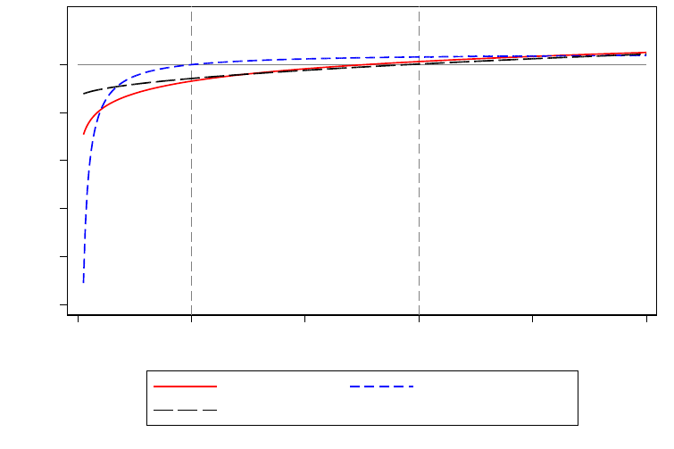
34
discount of 6.5%. Taken together, these results imply that a property inside the tsunami inundation zone
sells for 6.5 to 8.5% less than a property outside of the zone after the Tohoku event.
The Tohoku event is statistically significant in Model I (at the 5% significance level). Properties
sold after the Tohoku earthquake/tsunami sold for 9.0% more according to Model I. The New Yorker article
event is not statistically significant in either Model II or III. The coefficients on these event variables capture
the temporal effect for properties both inside and outside the tsunami inundation zone. This result indicates
that the average real value for all properties increased over time by approximately 9% between the Tohoku
earthquake and the New Yorker article but did not appreciably increase after the New Yorker article. The
coefficients on the SB 379 tsunami inundation zone treatment variable in Models I and III implies that
houses inside the SB 379 zone have a price premium of 6.4 to 6.9% (at the 10% significance level). This
suggests that the SB 379 zone treatment variable may be capturing the value of unobserved coastal
amenities. The coefficient on 2013 is not statistically significant.
As expected, house prices increase with elevation and with proximity to the ocean. These results
are statistically significant (at the 1% or 5% level) and signify the importance of coastal view amenities. I
interact these two variables for oceanfront homes in ln () to create a
proxy for ocean view. This proxy appears to have a positive and statistically significant effect (at the 1%
level) on property prices in all models. For oceanfront homes, as elevation increases and (log) distance to
Figure 7.
Decay effects of tsunami risk over time after the Tohoku earthquake and tsunami. Plot of coefficients from equation
(4) as in Bin and Landry (2013).
-50 -40
-30 -20 -10 0
Discount (%)
0
10 20 30 40 50
Months after 2011 Tohoku EQ
ln(Months) (Months-1)/Months
sqrt(Months)

35
the ocean shoreline increases (implying increasing beach width), sales prices increase. While this
interaction term has the expected sign, it does not fully capture the view amenity for oceanfront homes.
22
Following the finding of a statistically significant risk discount for the 2011 Tohoku earthquake
and tsunami, I test whether this risk discount decays over time. I find that three out of the four
transformations of the
(
)
variable in equation (4) had a positive and statistically significant
interaction with treatment, which is suggestive of a decay effect (at the 5% or 10% significance level).
23
Figure 7 plots the significant results as in Bin and Landry (2013) using the coefficients on the treatment
variable and on the interaction term between treatment and the
(
)
transformation. This figure
suggests that the risk premium decays between 10 months and 30 months after the Tohoku event. Thus, the
overall result for this analysis suggests that a property inside the SB 379 tsunami inundation zone sells for
6.5-8.5% less than a property outside of the zone after the Tohoku event but property prices inside the
inundation zone quickly return to baseline levels within 2.5 years of the Tohoku event.
Table 4 reports the results from the Oaxaca-Blinder decompositions. Recall that, like the DID
estimator, the unexplained component of the decomposition can be interpreted as the average treatment
effect on the treated (ATET) (Fortin et al., 2010; Słoczyński, 2015). Thus, the Oaxaca-Blinder estimator
suggests that there is an 8.9% risk discount for properties inside of the SB 379 inundation zone after the
Tohoku event (at the 5% significance level). The Oaxaca-Blinder estimator for the article event is not
statistically significant for Model II.
22
Further attempts to disentangle coastal amenities from tsunami risk involve using GIS viewshed tools and fine-scale digital
surface models of the ocean shoreline to calculate the view amenity for oceanfront homes. See section 7 for further details.
23
These results are not presented here but are available upon request.
Table 4. Oaxaca-Blinder results for the first analysis, full data
Model I
Model II
Coefficient/SE
Coefficient/ SE
Overall Differential
Treated group
12.457***
12.537***
(.0239)
(.0118)
Control group
12.451***
12.492***
(.0086)
(.0074)
Difference
.0063
.0449***
(.0254)
(.0139)
Decomposition
Explained
.0952**
.0385*
(.0386)
(.0231)
Unexplained
-.0889**
.0064
(.0391)
(.0231)
Observations
5890
9160
* p<0.10, ** p<0.05, *** p<0.01

36
Table 5 presents results from the event study regression for Models I and II. The lag variables
represent quarters prior to the event of interest and the lead variables represent quarters after the event, e.g.,
the 1 variable represents the first quarter after the event. As is standard, the first lag is omitted as a
baseline. For Model I, the sixth quarter lag variable is statistically significant, suggesting that there are
parallel pre-trends for at least 5 quarters before the Tohoku earthquake and tsunami. This result also
supports the parallel pre-trends observed graphically in Figure 5(a). The first quarter lead is statistically
significant but subsequent lead variables are not. This suggests there is a risk discount of 14.0% one quarter
after the Tohoku earthquake and tsunami but that this effect decays rapidly after the first quarter. This event
study estimator is slightly larger in magnitude than the full data OLS results and decays more rapidly.
However, the key outcome is that the risk discounts are in the same direction and relative magnitude. This
short-lived response supports the idea that the Tohoku event acted as a pure/distant information shock that
does not persist. For Model II, the lack of significance of any of the lag variables suggests that there are
parallel pre-trends for at least 8 quarters before the New Yorker article. The statistically significant results
for the post-event lead variables are conflicting. The variable for the quarter during which the event of
interest occurs (0) is positive and two quarters later the second lead variable is negative. Thus, the
event study results are inconclusive about the direction of the risk discount, which is complementary to the
full data OLS results that suggest a null result for Model II.
Appendix A.6 presents the covariate balance results for the PSM, NNM, CEM and EB
matching/weighting methods. The two matching methods (PSM and NNM) that improved covariate
Table 5. Event study results for the first analysis, full data
Model I
Model II
Coefficient
SE
Coefficient
SE
lag8
-.0581
(.1246)
-.0357
(.0537)
lag7
.0244
(.0663)
-.0325
(.0574)
lag6
.1344**
(.0622)
-.0113
(.0440)
lag5
.0899
(.0630)
-.0269
(.0404)
lag4
.0142
(.0599)
.0079
(.0381)
lag3
.0634
(.0602)
.0237
(.0399)
lag2
.0824
(.0603)
-.0006
(.0361)
lead0
.0609
(.0707)
.0603*
(.0318)
lead1
-.1399**
(.0682)
.0534
(.0364)
lead2
-.0212
(.0606)
-.0671*
(.0386)
lead3
-.0675
(.0659)
.0127
(.0353)
lead4
.0284
(.0632)
.0008
(.0354)
lead5
-.0372
(.0551)
.0007
(.0381)
lead6
.0267
(.0577)
-.0657
(.0429)
lead7
-.0056
(.0625)
-.0570
(.0395)
lead8
.0890
(.1266)
-.0134
(.0667)
Observations
5890
9160
Adj. R-squared
0.375
0.441
* p<0.10, ** p<0.05, *** p<0.01

37
balance for the key variables that likely influence treatment also dropped approximately 90% of the control
observations and the matching method (CEM) that does not drop most of the control observations also does
not appreciably improve covariate balance. EB, a pure weighting method, improved covariate balance for
the key matching variables but effectively “dropped” many control observations by assigning very small
weights to them. Due to these concerns the matched samples are not used to replace the original unmatched
data. Instead, I run the three primary models using the matched data from all four matching methods and
report these results in comparison to the full, unmatched data results.
Table 6 reports selected estimation results of the key coefficients for Models I through III using the
matched data. After PSM, the DID estimators are still statistically significant (at the 5% significance level)
for the 2011 Tohoku earthquake and tsunami in both Models I and III. The coefficient estimates suggest
that a property inside the SB 379 tsunami inundation zone has a risk discount of 10-12% following the
Tohoku event. After NNM, the DID estimator for the Tohoku event is suggestive of a 12% risk discount
(at the 5% significance level) for Model I but is no longer statistically significant for Model III. After CEM,
the DID estimator for the Tohoku event is suggestive of a 9% risk discount (at the 10% significance level)
Table 6. Difference-in-differences selected results, matched data
Model I
Model II
Model III
Matching method and Diff-in-Diff estimators
Coefficient/SE
Coefficient/SE
Coefficient/SE
Nearest neighbor propensity score (PSM)
SB 379 zone (sb379) x sold after 2011 Tohoku EQ (tohoku)
-.1224**
-.1056**
(.0530)
(.0426)
2013 XXL zone (xxl2013) x sold after 2015 article (article)
-.0389
(.0301)
SB 379 zone (sb379) x sold after 2015 article (article)
.0459
(.0297)
Nearest neighbor Mahalanobis (NNM)
SB 379 zone (sb379) x sold after 2011 Tohoku EQ (tohoku)
-.1236**
-.0165
(.0524)
(.0415)
2013 XXL zone (xxl2013) x sold after 2015 article (article)
-.0251
(.0279)
SB 379 zone (sb379) x sold after 2015 article (article)
6.7e-04
(.0293)
Coarsened exact matching (CEM)
SB 379 zone (sb379) x sold after 2011 Tohoku EQ (tohoku)
-.0649
-.0923*
(.0576)
(.0508)
2013 XXL zone (xxl2013) x sold after 2015 article (article)
-.0480
(.0427)
SB 379 zone (sb379) x sold after 2015 article (article)
.0371
(.0355)
Entropy balancing (EB)
SB 379 zone (sb379) x sold after 2011 Tohoku EQ (tohoku)
-.0685
-.0393
(.0509)
(.0410)
2013 XXL zone (xxl2013) x sold after 2015 article (article)
-.0173
(.0315)
SB 379 zone (sb379) x sold after 2015 article (article)
-.0086
(.0291)
* p<0.10, ** p<0.05, *** p<0.01

38
for Model III but is no longer statistically significant for Model I. After EB, the DID estimators are no
longer statistically significant for either Model I or III. The DID estimator for the 2015 New Yorker article
is not statistically significant in either Model II or III for any of the four methods. One issue with matching
is that there are few good controls with respect to the two key matching variables – elevation and distance
to the ocean – since assignment to the tsunami inundation zone is highly dependent on both variables. Thus,
all four matching/weighting methods assign high weights to few observations and low weights to many
observations, effectively “dropping” many control observations. This increases standard errors and
confidence intervals for the resulting post-matching DID coefficients. However, the post-matching
estimators all have similar magnitudes to the full data OLS results and the Oaxaca-Blinder results. Since
the post-matching results are consistent with the full data results, albeit with larger standard errors, matching
may not be important in this context.
The results of the four sets of falsification tests are presented in Table A10 of Appendix A.7. In all
four tests the DID estimates for Model I are smaller in magnitude compared to the main full data estimate
of 8.5% and are not statistically significant. The DID estimates for Model III and the 2011 Tohoku event
are also smaller in magnitude than the main estimate of 6.5% and are not statistically significant in all tests
(the fourth test does not apply to Model III). The 2015 New Yorker article event is still not statistically
significant in either Model II or III in all four tests. These falsification tests lend additional support to a
causal interpretation of the estimated risk discounts.
Figure 8 summarizes the results for the first analysis. It plots the average treatment effect on the
treated (ATET) estimates with 95% confidence intervals for Models I and II.
24
For each model, the full data
estimator is on the left. The next four points represent the estimators after the data was processed with the
four matching methods (PSM, NNM, CEM, and EB). “OB” represents the Oaxaca-Blinder estimator. The
final six estimators represent the full data estimator under different sample space assumptions. The sample
space is changed from within 1 mile of the tsunami inundation line to ½ mile and also to 2 miles to compare
the effects of decreasing and increasing the sample area, respectively. Similarly, I decrease the time range
from 2 years around the event of interest to 1 year around the event. Finally, I try extending the sample
space to the entire seven counties. Figure 8(a) plots the ATETs for Model I. The takeaway from this plot is
that the full data result is robust to the matching estimators, the Oaxaca-Blinder estimator, and to varying
the sample space: all of the ATETs for the 2011 Tohoku earthquake and tsunami have the expected negative
sign and approximately same magnitude as the coefficient from the full data results. Figure 8(b) plots the
ATETs for Model II and shows that the full data’s null result is robust to the matching estimators, the
24
See Figures A4(a) and A4(b) in Appendix A.7 for plots of the ATETs for Model III’s Tohoku event and New Yorker article
event, respectively. These results generally corroborate the results in Figures 8(a) and 8(b). For the Tohoku event, all of the ATETs
are negative and most (except the post-NNM estimator) are similar in magnitude to the full data estimate. For the New Yorker
article event, most of the ATETs including the full data estimate are not statistically significant.
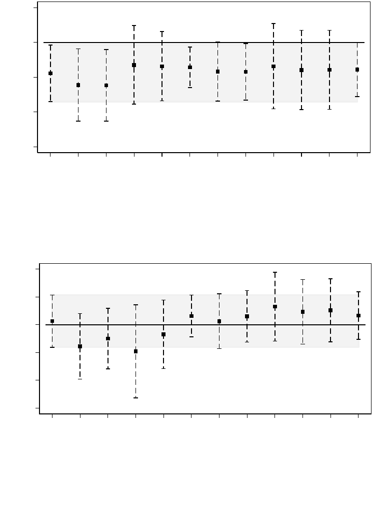
39
Oaxaca-Blinder estimator, and to varying the sample space: the ATETs for the 2015 New Yorker article
are not statistically significant for any of the presented models.
(a)
(b)
Figure 8.
Average treatment effect on the treated estimates with 95% confidence intervals for the first analysis’ models. The
full data estimator is on the left. The next four points represent the estimators after the data was processed with the four matching
methods (PSM, NNM, CEM, and EB). OB represents the Oaxaca-Blinder estimator. The final six estimators represent the full
data estimator under different sample space assumptions. (a) For Model I. (b) For Model II.
-.3 -.2 -.1 0 .1
Coefficients: sb379xtohoku
Full
PSM
NNM
CEM
EB
Oaxaca-Blinder
Full - 1/2 mile
Full - 2 miles
Full - 1/2 mile, 1 year
Full - 1 mile, 1 year
Full - 2 miles, 1 year
Full - 7 counties
Model
y
-.15 -.1 -.05
0 .05 .1
Coefficients: xxl2013xarticle
Full
PSM
NNM
CEM
EB
Oaxaca-Blinder
Full - 1/2 mile
Full - 2 miles
Full - 1/2 mile, 1 year
Full - 1 mile, 1 year
Full - 2 miles, 1 year
Full - 7 counties
Model
y
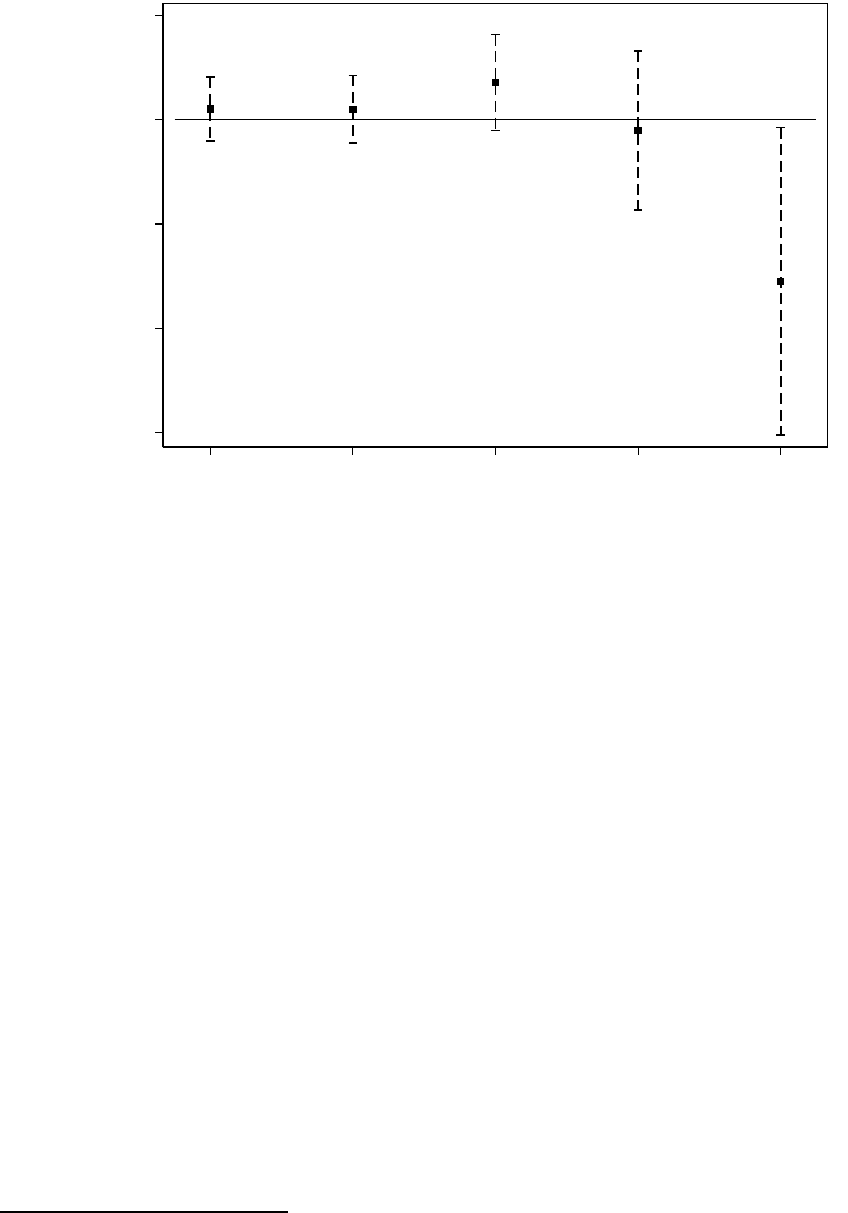
40
6.2 Second analysis: 2013 change in tsunami evacuation maps
For the second analysis, the DID coefficients for the XXL, XL, L or M tsunami inundation zones are not
statistically significant (Models 1-4). The DID coefficient for the smallest inundation zone is negative,
large, and statistically significant at the 5% level, implying that a property inside the 2013 SM tsunami
inundation zone has a risk discount of 26.6% following the 2013 map change. These results are summarized
in Figure 9, which plots the full data DID estimators with 95% confidence intervals for Models 1 through
5.
25
I also test whether the risk discount for the SM tsunami inundation zone decays over time and find that
none of the four transformations of the
(
)
variable in equation (4) had a statistically
significant interaction with treatment. This suggests that the risk discount does not have a statistically
significant decay effect.
The combined model with all five 2013 tsunami inundation zones supports the main DID results:
the only statistically significant DID coefficient is that of the smallest inundation zone.
26
This model implies
that a property inside the 2013 SM inundation zone has a risk discount of 23.9% following the 2013 map
change (at the 10% significance level). A robustness check with the Oaxaca-Blinder decomposition is not
statistically significant for the XXL, XL, L or M tsunami inundation zones (Models 1-4).
27
However, the
25
Table A11 of Appendix A.7 reports the full estimation results with all coefficients.
26
Table A12 of Appendix A.7 reports the combined model results.
27
Table A13 of Appendix A.7 reports the Oaxaca-Blinder results.
Figure 9. Average treatment effect on the treated estimates with 95% confidence intervals for Models 1 through 5 of the
second analysis.
-.6 -.4 -.2
0 .2
Coefficients
1 - XXL 2 - XL
3 - L 4 - M
5 - SM
y

41
Oaxaca-Blinder estimator is marginally significant for Model 5 and suggestive of a 17.2% risk discount for
properties inside the 2013 SM tsunami inundation zone following the 2013 map change (p-value = 0.1007).
I ran event study regressions for Model 5, the only model that had significant full data results, but there
were too few treated observations in some quarters to precisely estimate treatment effects in an event study
framework.
28
The results of the four sets of falsification tests are presented in Table A14 of Appendix A.7.
In all four tests the DID estimates for Model 5, the primary model of interest, are smaller in magnitude
compared to the main estimate of 26.6% and are not statistically significant.
29
This result supports the causal
interpretation of the risk discount found in Model 5. Combined, the OLS and Oaxaca-Blinder results suggest
that properties inside the SM inundation zone sold for 17-27% less after the 2013 map change.
6.3 Third analysis: Tsunami Blue Line project
The first step in this analysis required testing neighborhood sizes around the blue lines by running 100
models that vary the treatment buffer and control buffer radii. Figure 10 summarizes the results of these
tests. It plots the average treatment effect on the treated (ATET) estimates for the DID models with 95%
confidence intervals for Models 1 through 100 where each model is defined by the treatment buffer size
and control buffer size combination that determines its sample space. The 95% confidence intervals – and
the p-values used for hypothesis testing – were generated using subcluster wild bootstrapping, an extension
of the wild cluster bootstrap. Each municipality that installed blue lines was given a set of blue lines from
the state and chose themselves where to install these blue lines, meaning that the treatment assignment
mechanism is clustered by municipality. This suggests using cluster-robust standard errors. However, there
are only 8 to 15 municipalities (this varies by model), which is less than the recommended 40 to 50 clusters
(Angrist & Pischke, 2009). With too few clusters, the cluster-robust variance matrix estimate will be
downward-biased, leading to over-rejection of the null hypothesis (Cameron & Miller, 2015).
Bootstrapping diagnostics suggested that subcluster wild bootstrapping – clustering on both municipality
and year – performed better than ordinary wild cluster bootstrapping on municipality alone. Furthermore,
whereas the ordinary wild cluster bootstrap fails when cluster sizes vary, as is the case here, the subcluster
wild bootstrapping method has been shown to perform well when the number of clusters is small and when
cluster sizes vary (MacKinnon & Webb, 2018).
Models 1 through 50 (Figures A5(a) and A5(b) in Appendix A.7) use Euclidian distances and
Models 51 through 100 (Figures 10(a) and 10(b)) use road network distances to define the treatment and
28
These results are not presented here but are available upon request.
29
There are two unexpected and statistically significant results of the falsification tests. First, the DID estimates for Models 1 and
2 are marginally statistically significant in the first test (shifting the date of the 2013 map change to one year before the true event,
i.e., October 2012). Since some counties received updated tsunami maps in early 2013 these two models may be picking up the
treatment effect due to these early-adopting counties. Second, the DID estimates for Model 3 are statistically significant but positive
in the third test (randomly assigning sales to either the control or treatment group). This result is counterintuitive and likely an
artifact of the randomization.

42
control buffers. The models that use road network distances tend to have treatment effects that agree more
with each other within a given treatment buffer compared to the models that use Euclidian distances, which
possibly suggests that the road network distance models are more consistently picking up the effect of
proximity to a blue line. This makes intuitive sense since the blue lines are placed on roads that homeowners
drive on regularly to and from their properties. So, using the road network to measure distances between
properties and blue lines likely aligns better with how homeowners are perceiving these distances.
Therefore, I focus on the results road network models (Figures 10(a) and 10(b)).
Figure 10(a) shows the estimates for the 500’, 1000’, and 1500’ treatment buffers defined using
road network distances. The first nine model estimates in this figure are for the 500’ treatment buffer with
the control buffer expanding from 1000’ to 5000’. The next nine estimates are for the 1000’ treatment buffer
with the control buffer expanding from 1500’ to 5500’. The last nine estimates are for the 1500’ treatment
buffer with the control buffer expanding from 2000’ to 6000’. Figure 10(a) suggests that the 500’ treatment
buffer is too small – there are not enough observations to identify the treatment effect. The 1000’ treatment
buffer models all have negative effects, with several treatment effects having statistical significance. The
1500’ treatment buffer does not have any significant treatment effects. In fact, the treatment effect appears
to go to zero. Figure 10(b) shows the estimates for the 2000’, 2500’, and 3000’ treatment buffers. Combined,
these two figures suggest that when the treatment buffer is 1500’ or larger the treatment effect goes to zero.
The most significant results tend to be for smaller treatment buffers, specifically the 1000’ treatment buffer,
and these results are more significant for smaller control buffers, which is when the sets of treatment and
control buffer observations are the most comparable or balanced. As hypothesized, the treatment effect of
the blue lines is extremely localized. Thus, I narrow the spatial extent choice to the 1000’ treatment buffer.
Within this treatment buffer, I am simultaneously testing nine control buffers (Models 60 through
68) so I have to account for this multiple hypothesis testing.
30
I use the Simes correction to generate q-
values (adjusted p-values) for these nine models because it has several desirable features: it is not as
conservative as the traditional Bonferroni correction, it is a step-up method, and it allows for non-negative
correlation between the p-values (Newson, 2010). Step-up methods start with a single-step method (like the
Bonferroni correction) but then improve upon single-step methods by possibly rejecting further hypotheses
in subsequent steps (Romano et al., 2010). The q-value generated by the Simes procedure for Models 62
and 63 is 0.089.
31
This is the minimum proportion of false positive results (the false discovery rate) when
the test is significant, i.e., 8.9% of significant results will result in a false positive.
30
I could apply multiple hypothesis testing procedures to a larger subset of models but, as expected, the adjusted p-values are very
high.
31
The full set of q-values is not reported here but is available upon request.
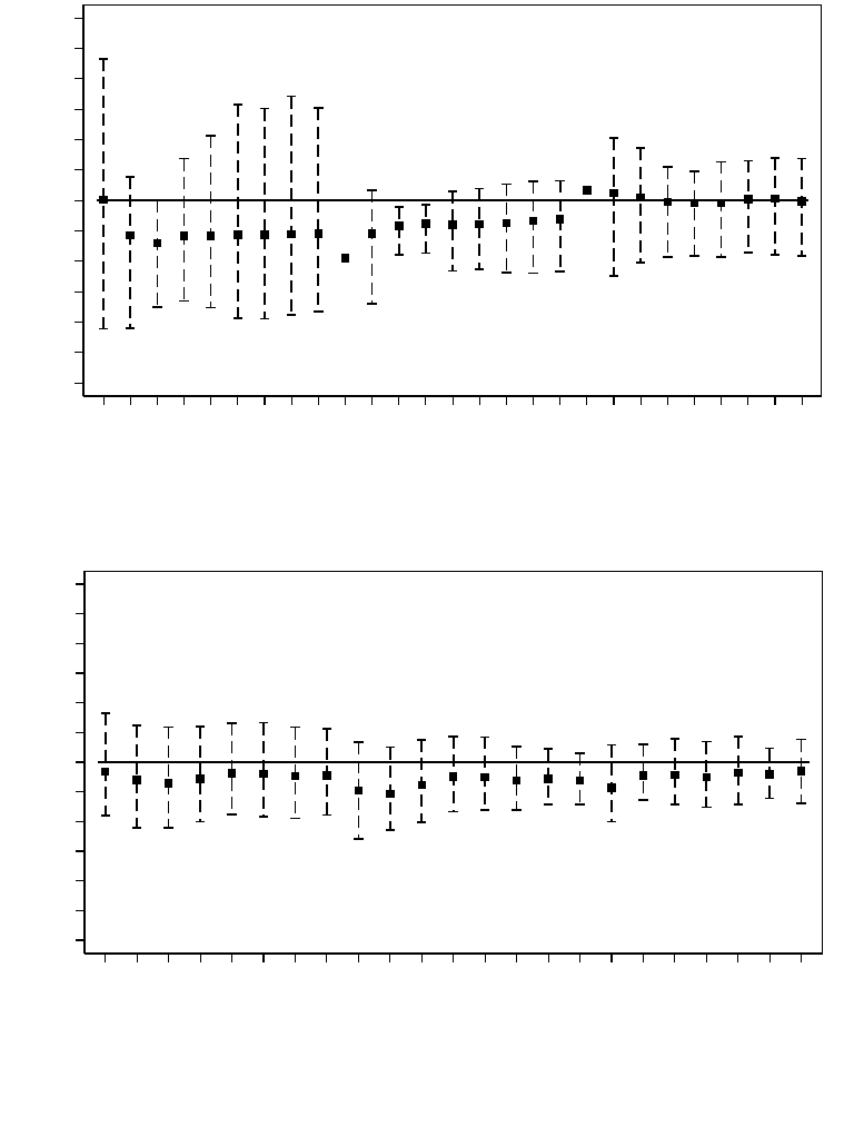
43
(a)
(b)
Figure 10.
Average treatment effect on the treated estimates with 95% confidence intervals for Models 51 through 100 of the
third analysis. Road network distances define the treatment and control buffers. For each ATET, the model number is followed
by the size of the treatment buffer (ft) and the size of the control buffer (ft), e.g., Model 51 has a 500’ treatment buffer and 1000’
control buffer. (a) For Models 51-77. (b) For Models 78-100. Note: confidence intervals that are out of bounds are suppressed,
e.g., for Model 60.
-.6 -.5 -.4 -.3 -.2 -.1
0 .1 .2 .3 .4 .5 .6
Coefficients
51 - 500, 1000
52 - 500, 1500
53 - 500, 2000
54 - 500, 2500
55 - 500, 3000
56 - 500, 3500
57 - 500, 4000
58 - 500, 4500
59 - 500, 5000
60 - 1000, 1500
61 - 1000, 2000
62 - 1000, 2500
63 - 1000, 3000
64 - 1000, 3500
65 - 1000, 4000
66 - 1000, 4500
67 - 1000, 5000
68 - 1000, 5500
69 - 1500, 2000
70 - 1500, 2500
71 - 1500, 3000
72 - 1500, 3500
73 - 1500, 4000
74 - 1500, 4500
75 - 1500, 5000
76 - 1500, 5500
77 - 1500, 6000
y ( )
-.6 -.5 -.4 -.3 -.2 -.1 0
.1 .2 .3 .4 .5 .6
Coefficients
78 - 2000, 3000
79 - 2000, 3500
80 - 2000, 4000
81 - 2000, 4500
82 - 2000, 5000
83 - 2000, 5500
84 - 2000, 6000
85 - 2000, 6500
86 - 2500, 3500
87 - 2500, 4000
88 - 2500, 4500
89 - 2500, 5000
90 - 2500, 5500
91 - 2500, 6000
92 - 2500, 6500
93 - 2500, 7000
94 - 3000, 4500
95 - 3000, 5000
96 - 3000, 5500
97 - 3000, 6000
98 - 3000, 6500
99 - 3000, 7000
100 - 3000, 8000
y ( )

44
Following these tests, I choose one model to continue the analysis with: Model 62.
32
It has a 1000’
treatment buffer and a 2500’ control buffer. Table 7 reports selected DID and DDD estimation results of
the key coefficients for Model 62.
33
The DID estimator suggests that there is an 8.0% risk discount for
properties that are within 1000’ of a blue line (at the 5% significance level, uncorrected). The DDD
estimator is not statistically significant, however. These results suggest homebuyers attend to the visual
cues but do not differentiate the signal according to the classification of tsunami inundation risk. The
treatment and event variables are not statistically significant in either the DID or DDD model. The
sensitivity variable for the 2013 XXL tsunami inundation zone is statistically significant (at the 10% level)
in the DDD model, suggesting that houses inside the 2013 XXL inundation zone sell for 14.6% more than
houses outside of it. This variable may be capturing the value of unobserved coastal amenities. In both the
DID and DDD models house prices increase with proximity to the ocean (at the 1% significance level).
32
Once this model is selected, subsequent p-values are generated using the subcluster wild bootstrapping procedure and are not
corrected for multiple testing procedures.
33
Table A15 of Appendix A.7 reports the full estimation results with all coefficients.
Table 7. Difference-in-differences and triple differences results for the third analysis, Model 62
DID
DDD
Coefficient
p-
value
Coefficient
p-value
Treatment
Blue line treatment buffer (treatment362=1)
.0218
.4658
.0398
.2532
Event
Sold after first blue line installed (event362=1)
.0185
.8296
.1012
.7396
Sensitivity
Inside 2013 XXL tsunami zone (xxl2013=1)
.1365*
.0800
Diff-in-Diff
Blue line treatment buffer (treatment362) x sold after first blue
line installed (event362)
-.0834**
.0254
-.0832
.4731
Blue line treatment buffer (treatment362) x 2013 XXL zone
(xxl2013)
-.0623
.3290
2013 XXL zone (xxl2013) x sold after first blue line installed
(event362)
-.2488
.1507
Triple Difference
Blue line treatment buffer x 2013 XXL zone x sold after first
blue line installed
-.0117
.9404
Location
Elevation (ft)
5.9e-04
.2038
.0011
.1197
Elevation (ft) x Log distance to ocean shoreline x on oceanfront
(=1)
2.9e-04
.2527
2.8e-04
.2660
Log distance to ocean shoreline
-.0799***
.0081
-.0747***
.0088
Observations
1334
1334
Adj. R-squared
0.491
0.496
* p<0.10, ** p<0.05, *** p<0.01
45
However, elevation and the ocean view proxy ln () are no longer
statistically significant in either the DID or DDD model.
Next, I calculate the measure proposed by de Chaisemartin and D’Haultfœuille (2020) to assess the
robustness of the TWFE estimator to heterogeneous treatment effects. This robustness measure is the ratio
of the TWFE estimator to the standard deviation of the weights attached to the TWFE regression (de
Chaisemartin & D’Haultfœuille, 2020). If this ratio is very large, the TWFE estimator and the ATET can
only be of opposite signs under a very large and implausible amount of treatment effect heterogeneity.
However, if many weights are negative, and if the robustness measure is not very large (close to 0), the
TWFE estimator and the ATET can be of opposite signs even under a small and plausible amount of
treatment effect heterogeneity. The calculated robustness measure (0.0103) for Model 62 suggests that
treatment effect heterogeneity could be a serious concern for the validity of the TWFE estimator.
Following this result, I estimate two new estimators that are valid in the presence of treatment effect
heterogeneity. I first compute new DID estimator by de Chaisemartin and D’Haultfœuille (2020) that
estimates the treatment effect in the groups that switch treatment, at the time when they switch. I find a
large, negative but not statistically significant effect (
= 0. 392, = 0. 664). I then run a new
estimator developed by Callaway and Sant’Anna (2020) whose interpretation is similar to the ATET in the
TWFE DID setup. However, the data for Model 62 is too sparse to be able to estimate most of their group-
time average treatment effects. Out of seven groups, I can calculate group average treatment effects for
only two groups and, while negative, these group average treatment effects are not statistically significant.
There are also too many missing group average treatment effects to calculate an overall treatment effect
that could be compared to the TWFE DID estimator. The treatment effects generated by these new methods
have the same sign as TWFE but the magnitudes and significance are likely impacted by the small sample
in this rural location.
7 Discussion and Conclusion
The Pacific Northwest is facing a severe but low frequency threat: the Cascadia Subduction Zone (CSZ)
earthquake and tsunami. In Oregon, resilience to such a large seismic event is low and coastal communities
in the tsunami inundation zone are especially vulnerable. They will account for the majority of expected
fatalities and those who survive will be instantly displaced (OSSPAC, 2013; Schulz, 2015b). Whether
individual Oregonians will take action to prepare themselves for a CSZ event depends on how salient the
risk is. Since Oregon has not experienced a Cascadia earthquake and tsunami in recent history, Oregonians’
subjective risk perceptions may underestimate the objective probability of a Cascadia event. This study
asks whether new information about the risk of a Cascadia earthquake and tsunami can narrow the gap
between subjective and objective risk.
46
The results for the first analysis on exogenous events suggest that a property inside the SB 379
tsunami inundation zone sells for 6.5-8.5% less than a property outside of the zone after the 2011 Tohoku
earthquake and tsunami. However, this risk discount is short-lived and properties inside the SB 379
inundation zone return to baseline levels within 2.5 years of the Tohoku event. The DID estimator for the
2015 New Yorker article is not statistically significant in either Model II or III. The 2011 Tohoku
earthquake and tsunami treatment effect is robust to the Oaxaca-Blinder estimator, matching estimators,
and an event study specification.
For the second analysis on regulatory map changes, the DID estimators are statistically significant
for the 2013 SM tsunami inundation zone but not for the M, L, XL, or XXL zones. The coefficient estimate
from Model 5 implies that a property inside the SM inundation zone has a risk discount of 26.6% following
the 2013 map change. Thus a risk discount may exist for homes that were not in the original 1995 tsunami
inundation zone but are in the most vulnerable 2013 inundation zone – and therefore all of the new
inundation zones – following the 2013 map update. This result is robust to the Oaxaca-Blinder estimator,
which suggests a more conservative risk discount of 17.2%.
DID results from the third analysis on local visual risk cues using a 1000’ treatment buffer and a
2500’ control buffer suggest an 8.0% risk discount for properties that are within 1000’ of a blue line. This
result could be invalidated by the presence of treatment effect heterogeneity, a potential concern for this
analysis. However, the sample composed of small, rural communities limits my ability to verify the results
from the TWFE regression with the newly developed estimators that account for treatment effect
heterogeneity. When I run these new estimators, they are suggestive of a negative effect of proximity to a
blue line but, again, are not able to be estimated precisely. The DDD results from the third analysis are not
statistically significant, suggesting that people are not sensitive to whether they are inside the tsunami
inundation zone. Homeowners may not perceive a difference in risk if they’re immediately across the
inundation zone, e.g., they may think the water will reach their property even if they are outside of the
inundation zone since the zone is a modeled result and cannot be perfectly predictive. This result suggests
that people may attend to the visual cue given by the blue lines but not to the risk signal given by the tsunami
inundation zone. The third analysis has several next steps that are in progress. First, I need to include
recently acquired housing transactions for the years 2019 and 2020. This may help with some of the data
limitations in this analysis and may even make it possible to calculate the de Chaisemartin and
D’Haultfœuille (2020) and Callaway and Sant’Anna (2020) estimators. Second, since pre-tests based on
the group-time average treatment effects of Callaway and Sant’Anna (2020) are valid even if there is
variation in treatment timing, if additional data makes it possible to calculate this estimator then another
possible step for this analysis is to use this estimator to test for parallel pre-trends.
47
Many of the limitations of these three analyses are due to limited observations or covariates. In the
first analysis, the positive coefficients on the SB 379 tsunami inundation zone treatment variable suggest
that it is capturing the value of unobserved coastal amenities. One promising attempt to disentangle coastal
amenities from tsunami risk involves using GIS viewshed tools and fine-scale digital surface models of the
ocean shoreline to calculate the view amenity for oceanfront homes (Bin et al., 2008; Dundas, 2017). There
may also be unobservable factors that influence the price trend for oceanfront properties. More data may
be needed to fully account for the unobserved coastal amenities driving location choice and potentially
confounding results. Similarly, for the second analysis, an ocean view covariate for oceanfront homes may
help this analysis better disentangle coastal amenities from tsunami risk. There are two potential concerns
with second analysis’ primary SM inundation zone result. First, for there are only 81 homes that fall into
the treatment group, i.e., were not in the SB 379 zone but are in the 2013 SM zone, for Model 5. Another
concern is the substantial covariate imbalance for this sample (see Table A3 of Appendix A.3). However,
the small sample size for this model precluded using any of the four matching methods to preprocess the
data as a robustness check.
The potential risk discounts identified in this paper indicate that at least three types of tsunami risk
signals – exogenous events, hazard planning changes, and visual cues – may be salient to coastal residents.
These results suggest that exogenous tsunami risk signals may shift homebuyers’ subjective risk perceptions
to better match the objective risks of the Cascadia event, meaning that a salient risk signal may be able to
successfully induce individuals to take preparedness actions. And given that Oregon is currently and
chronically under-prepared for a Cascadia earthquake and tsunami, policymakers and emergency managers
face the dual policy challenge of increasing the risk salience and preparedness action. Thus, more and better
policies – or risk signals – that encourage preparedness action are needed.
48
8 References
Angrist, J. D., & Pischke, J.-S. (2009). Mostly Harmless Econometrics: An Empiricist’s Companion (1st
ed.). Princeton University Press.
Atreya, A., & Ferreira, S. (2015). Seeing is Believing? Evidence from Property Prices in Inundated Areas.
Risk Analysis, 35(5), 828–848. https://doi.org/10.1111/risa.12307
Atreya, A., Ferreira, S., & Kriesel, W. (2013). Forgetting the Flood? An Analysis of the Flood Risk
Discount over Time. Land Economics, 89(4), 577–596. https://doi.org/10.3368/le.89.4.577
Baker, A., Larcker, D. F., & Wang, C. C. Y. (2021). How Much Should We Trust Staggered Difference-
In-Differences Estimates? (Rock Center for Corporate Governance at Stanford University
Working Paper No. 246). Rock Center for Corporate Governance, Stanford University.
https://doi.org/10.2139/ssrn.3794018
Bakkensen, L. A., Ding, X., & Ma, L. (2019). Flood Risk and Salience: New Evidence from the Sunshine
State. Southern Economic Journal, 85(4), 1132–1158. https://doi.org/10.1002/soej.12327
Beron, K. J., Murdoch, J. C., Thayer, M. A., & Vijverberg, W. P. M. (1997). An Analysis of the Housing
Market before and after the 1989 Loma Prieta Earthquake. Land Economics, 73(1), 101.
https://doi.org/10.2307/3147080
Bin, O., Kruse, J. B., & Landry, C. E. (2008). Flood Hazards, Insurance Rates, and Amenities: Evidence
From the Coastal Housing Market. Journal of Risk & Insurance, 75(1), 63–82.
https://doi.org/10.1111/j.1539-6975.2007.00248.x
Bin, O., & Landry, C. E. (2013). Changes in implicit flood risk premiums: Empirical evidence from the
housing market. Journal of Environmental Economics and Management, 65(3), 361–376.
https://doi.org/10.1016/j.jeem.2012.12.002
Blinder, A. S. (1973). Wage Discrimination: Reduced Form and Structural Estimates. The Journal of
Human Resources, 8(4), 436. https://doi.org/10.2307/144855
Borusyak, K., & Jaravel, X. (2017). Revisiting Event Study Designs, with an Application to the Estimation
of the Marginal Propensity to Consume [Unpublished Manuscript].
Brookshire, D. S., Thayer, M. A., Tschirhart, J., & Schulze, W. D. (1985). A Test of the Expected Utility
Model: Evidence from Earthquake Risks. Journal of Political Economy, 93(2), 369–389.
https://doi.org/10.1086/261304
Brown, T. T., & Atal, J. P. (2019). How robust are reference pricing studies on outpatient medical
procedures? Three different preprocessing techniques applied to difference-in differences. Health
Economics, 28(2), 280–298. https://doi.org/10.1002/hec.3841
Caliendo, M., & Kopeinig, S. (2008). Some Practical Guidance for the Implementation of Propensity
Score Matching. Journal of Economic Surveys, 22(1), 31–72. https://doi.org/10.1111/j.1467-
6419.2007.00527.x
Callaway, B., & Sant’Anna, P. H. C. (2020). Difference-in-Differences with multiple time periods.
Journal of Econometrics, S0304407620303948. https://doi.org/10.1016/j.jeconom.2020.12.001
Cameron, A. C., & Miller, D. L. (2015). A Practitioner’s Guide to Cluster-Robust Inference. Journal of
Human Resources, 50(2), 317–372. https://doi.org/10.3368/jhr.50.2.317
Cheng, A. S. (2018). Division of Financial Regulation 2017 Earthquake Insurance Data Call (p. 9).
Oregon Department of Consumer and Business Services.
Crowe, J. H. (2018). The Article That Shook the Public: In C. V. Fletcher & J. Lovejoy (Eds.), Natural
Disasters and Risk Communication: Implications of the Cascadia Subduction Zone Megaquake
(pp. 89–120). Lexington Books.
de Chaisemartin, C., & D’Haultfœuille, X. (2020). Two-Way Fixed Effects Estimators with
Heterogeneous Treatment Effects. American Economic Review, 110(9), 2964–2996.
https://doi.org/10.1257/aer.20181169
Department of Land Conservation & Development. (n.d.). Goal 18: Beaches and Dunes. Retrieved April
29, 2019, from https://www.oregon.gov/lcd/OP/Pages/Goal-18.aspx
49
Division of Financial Regulation. (n.d.). Earthquake insurance. Retrieved November 9, 2018, from
https://www.oregon.gov/oem/hazardsprep/Pages/2-Weeks-Ready.aspx
DOGAMI. (n.d.-a). Tsunami Inundation Map (TIM) Series. Retrieved February 11, 2019, from
https://www.oregongeology.org/pubs/tim/p-TIM-overview.htm
DOGAMI. (n.d.-b). Tsunami Regulatory Maps (Oregon Senate Bill 379) for the State of Oregon.
Retrieved February 11, 2019, from https://www.oregongeology.org/tsuclearinghouse/pubs-
regmaps.htm
DOGAMI. (2013, October 2). Tsunami inundation scenario data released for entire Oregon coast.
https://www.oregongeology.org/pubs/nr/press-release-2013-10-02.pdf
Dundas, S. J. (2017). Benefits and ancillary costs of natural infrastructure: Evidence from the New Jersey
coast. Journal of Environmental Economics and Management, 85, 62–80.
https://doi.org/10.1016/j.jeem.2017.04.008
Dundas, S. J., & Lewis, D. J. (2020). Estimating Option Values and Spillover Damages for Coastal
Protection: Evidence from Oregon’s Planning Goal 18. Journal of the Association of
Environmental and Resource Economists. https://doi.org/10.1086/708092
Fletcher, C. V., & Lovejoy, J. (2018). Natural Disasters and Risk Communication: Implications of the
Cascadia Subduction Zone Megaquake. Lanham, Maryland : Lexington Books.
Fontaine, L. (2016, August 24). New blue lines mark tsunami safe zones. The Astorian.
https://www.dailyastorian.com/news/local/new-blue-lines-mark-tsunami-safe-
zones/article_1e55aed0-581e-5c42-bf07-a91ae10c2d2a.html
Fortin, N., Lemieux, T., & Firpo, S. (2010). Decomposition Methods in Economics (No. w16045).
National Bureau of Economic Research. https://doi.org/10.3386/w16045
Gallagher, J. (2014). Learning about an Infrequent Event: Evidence from Flood Insurance Take-Up in the
United States. American Economic Journal: Applied Economics, 6(3), 206–233.
https://doi.org/10.1257/app.6.3.206
Gibson, M., & Mullins, J. T. (2020). Climate Risk and Beliefs in New York Floodplains. Journal of the
Association of Environmental and Resource Economists, 7(6), 1069–1111.
https://doi.org/10.1086/710240
Goodman-Bacon, A. (2018). Difference-in-Differences with Variation in Treatment Timing (No. w25018;
p. w25018). National Bureau of Economic Research. https://doi.org/10.3386/w25018
Google Trends. (n.d.). Google Trends. Retrieved November 9, 2018, from /trends/explore
Gu, T., Nakagawa, M., Saito, M., & Yamaga, H. (2018). Public Perceptions of Earthquake Risk and the
Impact on Land Pricing: The Case of the Uemachi Fault Line in Japan. The Japanese Economic
Review, 69(4), 374–393. https://doi.org/10.1111/jere.12173
Hainmueller, J. (2012). Entropy Balancing for Causal Effects: A Multivariate Reweighting Method to
Produce Balanced Samples in Observational Studies. Political Analysis, 20(1), 25–46.
https://doi.org/10.1093/pan/mpr025
Hallstrom, D. G., & Smith, V. K. (2005). Market responses to hurricanes. Journal of Environmental
Economics and Management, 50(3), 541–561. https://doi.org/10.1016/j.jeem.2005.05.002
Hanley, N., Shogren, J. F., & White, B. (Benedict). (2007). Environmental economics: In theory and
practice (2nd ed.). Basingstoke England.
Hansen, J. L., Benson, E. D., & Hagen, D. A. (2006). Environmental Hazards and Residential Property
Values: Evidence from a Major Pipeline Event. Land Economics, 82(4), 529–541.
https://doi.org/10.3368/le.82.4.529
Hastie, M. (Ed.). (2019). Clatsop County Housing Strategies Report (p. 40).
Ho, D. E., Imai, K., King, G., & Stuart, E. A. (2007). Matching as Nonparametric Preprocessing for
Reducing Model Dependence in Parametric Causal Inference. Political Analysis, 15(3), 199–236.
https://doi.org/10.1093/pan/mpl013
Iacus, S. M., King, G., & Porro, G. (2011). Multivariate Matching Methods That Are Monotonic
Imbalance Bounding. Journal of the American Statistical Association, 106(493), 345–361.
https://doi.org/10.1198/jasa.2011.tm09599
50
Iacus, S. M., King, G., & Porro, G. (2012). Causal Inference without Balance Checking: Coarsened Exact
Matching. Political Analysis, 20(1), 1–24. https://doi.org/10.1093/pan/mpr013
Imbens, G. W. (2004). Nonparametric Estimation of Average Treatment Effects under Exogeneity: A
Review. The Review of Economics and Statistics, 86(1), 4–29.
Jann, B. (2008). The Blinder–Oaxaca Decomposition for Linear Regression Models. The Stata Journal:
Promoting Communications on Statistics and Stata, 8(4), 453–479.
https://doi.org/10.1177/1536867X0800800401
Jung, H. (2011, March 11). Oregon officials express relief that tsunami passes by, then it hits the south
coast. OregonLive.Com. http://www.oregonlive.com/pacific-northwest-
news/index.ssf/2011/03/oregon_officials_express_relief_that_tsunami_passes_by_then_it_hits_th
e_south_coast.html
Kask, S. B., & Maani, S. A. (1992). Uncertainty, Information, and Hedonic Pricing. Land Economics,
68(2), 170. https://doi.org/10.2307/3146772
Kline, P. (2011). Oaxaca-Blinder as a Reweighting Estimator. American Economic Review, 101(3), 532–
537. https://doi.org/10.1257/aer.101.3.532
Kousky, C. (2010). Learning from Extreme Events: Risk Perceptions after the Flood. Land Economics,
86(3), 395–422. https://doi.org/10.3368/le.86.3.395
Kuminoff, N. V., & Pope, J. C. (2014). Do “Capitalization Effects” For Public Goods Reveal The
Public’s Willingness To Pay?: Do Capitalization Effects Reveal WTP? International Economic
Review, 55(4), 1227–1250. https://doi.org/10.1111/iere.12088
Kustura, A. (2016, March 11). Tsunami Blue Line Project: “You have to know your route to high
ground.” KMTR. https://nbc16.com/news/local/tsunami-blue-line-project-you-have-to-know-
your-route-to-high-ground
Lacitis, E. (2015, July 21). Ready—Or not? Earthquake kits flying off the shelves. The Seattle Times.
https://www.seattletimes.com/seattle-news/ready-or-not-earthquake-kits-flying-off-the-shelves/
Lovejoy, J. (2018). Conceptualizing Risk. In C. V. Fletcher & J. Lovejoy (Eds.), Natural Disasters and
Risk Communication: Implications of the Cascadia Subduction Zone Megaquake (pp. 1–12).
Lexington Books.
MacKinnon, J. G., & Webb, M. D. (2018). The wild bootstrap for few (treated) clusters. The
Econometrics Journal, 21(2), 114–135. https://doi.org/10.1111/ectj.12107
Marum, A. (2016, April 18). New Yorker writer wins Pulitzer for “The Really Big One”, thanks Steve
Novick. OregonLive.Com.
http://www.oregonlive.com/today/index.ssf/2016/04/really_big_one_pulitzer_new_yorker.html
McCluskey, J. J., & Rausser, G. C. (2001). Estimation of Perceived Risk and Its Effect on Property
Values. Land Economics, 77(1), 42–55. https://doi.org/10.2307/3146979
McCoy, S. J., & Walsh, R. P. (2018). Wildfire risk, salience & housing demand. Journal of
Environmental Economics and Management, 91, 203–228.
https://doi.org/10.1016/j.jeem.2018.07.005
Muehlenbachs, L., Spiller, E., & Timmins, C. (2015). The Housing Market Impacts of Shale Gas
Development. American Economic Review, 105(12), 3633–3659.
https://doi.org/10.1257/aer.20140079
Nakanishi, H. (2017). Quasi-experimental evidence for the importance of accounting for fear when
evaluating catastrophic events. Empirical Economics, 52(2), 869–894.
https://doi.org/10.1007/s00181-016-1084-6
Naoi, M., Seko, M., & Sumita, K. (2009). Earthquake risk and housing prices in Japan: Evidence before
and after massive earthquakes. Regional Science and Urban Economics, 39(6), 658–669.
https://doi.org/10.1016/j.regsciurbeco.2009.08.002
Newson, R. B. (2010). Frequentist Q-values for Multiple-test Procedures. The Stata Journal, 10(4), 568–
584. https://doi.org/10.1177/1536867X1101000403
Oaxaca, R. L. (1973). Male-Female Wage Differentials in Urban Labor Markets. International Economic
Review, 14(3), 693. https://doi.org/10.2307/2525981
51
Office of Emergency Management. (2016, February 16). Oregon Tsunami Blue Line Project Kicks Off.
https://www.oregon.gov/newsroom/Pages/NewsDetail.aspx?newsid=1221
Oregonian, T. (2019, June 24). Oregon Legislature repeals ban on building in tsunami zone. Oregonlive.
https://www.oregonlive.com/politics/2019/06/oregon-legislature-repeals-ban-on-building-in-
tsunami-zone.html
OSSPAC. (2013). The Oregon Resilience Plan: Reducing Risk and Improving Recovery for the Next
Cascadia Earthquake and Tsunami [Report to the 77th Legislative Assembly].
OSSPAC. (2018). Encouraging Homeowner Resilience through Earthquake Insurance and Seismic
Retrofit (OSSPAC Publication No. 18–01; p. 40).
Parton, L. C., & Dundas, S. J. (2020). Fall in the sea, eventually? A green paradox in climate adaptation
for coastal housing markets. Journal of Environmental Economics and Management, 102381.
https://doi.org/10.1016/j.jeem.2020.102381
Preparedness Framework Implementation Team (Prep-FIT). (n.d.). Emergency Preparedness Data
Collection (OR-IRIS Geodatabase and Mapfile). Retrieved February 11, 2019, from
https://spatialdata.oregonexplorer.info/geoportal/details;id=165d6af382ec435fb3faa3ca6e0c2736
Qiu, Y., & Gopalakrishnan, S. (2018). Shoreline defense against climate change and capitalized impact of
beach nourishment. Journal of Environmental Economics and Management, 92, 134–147.
https://doi.org/10.1016/j.jeem.2018.08.013
Romano, J. P., Shaikh, A. M., & Wolf, M. (2010). Multiple Testing. In Palgrave Macmillan (Ed.), The
New Palgrave Dictionary of Economics (pp. 1–5). Palgrave Macmillan UK.
https://doi.org/10.1057/978-1-349-95121-5_2914-1
Rosen, S. (1974). Hedonic Prices and Implicit Markets: Product Differentiation in Pure Competition.
Journal of Political Economy, 82(1), 34–55.
Schulz, K. (2015a, July 13). The Earthquake That Will Devastate the Pacific Northwest.
https://www.newyorker.com/magazine/2015/07/20/the-really-big-one
Schulz, K. (2015b, July 28). How to Stay Safe When the Big One Comes.
https://www.newyorker.com/tech/elements/how-to-stay-safe-when-the-big-one-comes
Secretary of State. (n.d.-a). City Populations. Retrieved February 11, 2019, from
https://sos.oregon.gov/blue-book/Pages/local/city-population.aspx
Secretary of State. (n.d.-b). County Populations. Retrieved February 3, 2019, from
https://sos.oregon.gov/blue-book/Pages/local/county-population.aspx
Sheeler, A. (2018, September 30). City of Coos Bay installs first tsunami Blue Line. The Coos Bay World.
https://theworldlink.com/news/local/city-of-coos-bay-installs-first-tsunami-blue-
line/article_5663918e-737b-51e8-8983-b3143fa08a1e.html
Słoczyński, T. (2015). The Oaxaca-Blinder Unexplained Component as a Treatment Effects Estimator.
Oxford Bulletin of Economics and Statistics, 77(4), 588–604. https://doi.org/10.1111/obes.12075
Stuart, E. A. (2010). Matching Methods for Causal Inference: A Review and a Look Forward. Statistical
Science, 25(1), 1–21. https://doi.org/10.1214/09-STS313
Sun, L., & Abraham, S. (2020). Estimating dynamic treatment effects in event studies with heterogeneous
treatment effects. Journal of Econometrics, S030440762030378X.
https://doi.org/10.1016/j.jeconom.2020.09.006
Tobias, L. (2012, March 11). One year after the Japanese tsunami, Oregon and California coastal towns
still learning, recovering. OregonLive.Com. http://www.oregonlive.com/pacific-northwest-
news/index.ssf/2012/03/one_year_after_the_japanese_ts.html
Totten, M. J. (2019). Off the Richter Scale. City Journal, Winter 2019. https://www.city-
journal.org/pacific-earthquakes
Wachinger, G., Renn, O., Begg, C., & Kuhlicke, C. (2013). The Risk Perception Paradox-Implications for
Governance and Communication of Natural Hazards: The Risk Perception Paradox. Risk
Analysis, 33(6), 1049–1065. https://doi.org/10.1111/j.1539-6924.2012.01942.x
Wood, N. (2007). Variations in City Exposure and Sensitivity to Tsunami Hazards in Oregon (Scientific
Investigations Report No. 2007–5283; p. 43). USGS.
52
Zillow. (2020). ZTRAX: Zillow Transaction and Assessor Dataset, 2020-Q4. Zillow Group, Inc.
http://www.zillow.com/ztrax/

53
A. Online Appendix
A.1 Expected utility model modified from Hallstrom and Smith (2005)
Using the expected utility framework, a person’s willingness to pay for a risk reduction captures the value
of risk reduction (conditional on their previous actions to reduce risk) (Hanley et al., 2007). A simple, two
outcome expected utility model, modified from Hallstrom and Smith (2005), demonstrates this in the case
of an earthquake and tsunami risk. Assume a person’s utility is given by the expected value of their utility
of wealth (income). Indirect utility
(
.
)
is defined over annual income minus any hazard insurance () and
the vector of housing attributes. This vector is decomposed into , the housing and site attributes that are
not related to the coastal amenities or risks, and , the site attribute that relates to both the
earthquake/tsunami risk and coastal amenities (such as distance to the shoreline). The household’s
subjective probability for an earthquake and tsunami at a given location (measured by distance ), with a
specific information set (), and state-contingent utility
(
.
)
is given by (, ). Their subjective
probability of no earthquake and tsunami is (1 (, )). Information, , can change due to preparedness
programs, media coverage, or the occurrence of earthquakes or tsunamis. In this two-outcome scenario, a
homeowner’s expected utility is given by
() =
(
,
)
, , , ,
,
(
,
)
(, ,
)
+1
(
,
)
, , , ,
,
(
,
)
,
(
. 1
)
where (. ) is the annual hedonic price function,
is the insurance rate per dollar of coverage, and is the
monetary loss due to the earthquake and tsunami, net of any insurance coverage. The state where the
earthquake and tsunami occurs is labeled () and the state where no earthquake occurs is (). Individuals
maximize their expected utility by selecting a house with attributes and conditional on their income
(), information (), insurance rates
(
)
, and the exogenous price function for these site attributes ((. )).
Assuming that this hedonic price function is the outcome of housing market equilibrium, we can
differentiate it with respect to an attribute of choice to find the implicit marginal price (marginal
capitalization effect) for that attribute. However, Hallstrom and Smith (2005) showed that it is difficult to
disentangle and interpret estimates for the marginal effect of (
=
) because distance () serves as a
proxy for both coastal amenities and risks of tsunami damage. They then show that observing the response
of housing prices to an exogenous information shock (
=
), instead, has the potential to reduce
confounding multiple influences on the marginal effect. Intuitively, a change in information changes the
individual’s perceived probability of an earthquake/tsunami
(
,
)
. This probability change (
) is
converted into a monetary tradeoff via the implicit price function. So, with an exogenous information shock

54
(), the marginal price from the hedonic isolates the ex ante marginal capitalization effect of the
information-induced change in subjective risk
=
=
(
)
+
(
1
)
, (. 2)
where
(
)
is the “incremental option price” for a unit risk reduction in the hazard (T) and
is the change in the perceived probability of an earthquake and tsunami due to the information shock .
34
Under my hypothesis that the tsunami risk signals – or information shocks – impacted Oregonians’ risk
perceptions about the Cascadia earthquake and tsunami, the sign of the ex ante marginal capitalization
effect (
) is expected to be negative for all information shocks. I expect that each information shock ()
increased individual’s perceived probability of an earthquake/tsunami
(
,
)
. The change in perceived risk
(
) should then decrease the hedonic price function (, ,
,
(
,
)
).
A.2 Tsunami inundation zone scenario comparison
Figure A1(a) presents the five 2013 tsunami inundation scenarios for the town of Tillamook, the Tillamook
County seat of 4,935 people (Secretary of State, n.d.-a). The five scenarios are known as the SM, M, L, XL,
and XXL tsunami inundation scenarios. Figure A1(b) compares the SM and XXL 2013 scenarios (blue) to
the 1995 SB 379 (orange) scenario for Tillamook. The differences between the two map series reflect the
differences in scientific information and modeling effort between 1995 and 2013. Figure A2 maps the
Census block groups for this same area in Tillamook to illustrate the approximate scale of a Census block
group for this sample.
34
Note that what I am calling the “incremental option price,” i.e., the maximum payment that an individual would make under
uncertainty to reduce the probability of the earthquake and tsunami state, is the term that converts the change in probability into
monetary terms. Also note that calling this term “incremental option price” is no longer technically correct since we are not able to
interpret the marginal effects of the hedonic price function as MWTP. For conciseness, I keep its original label here.
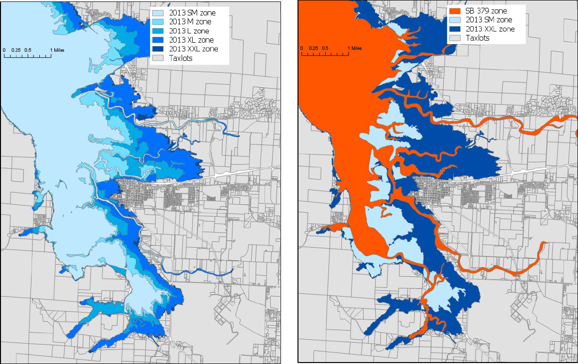
55
(a) (b)
Figure A1.
City of Tillamook, Tillamook County. (a) Tsunami inundation zones given by the five 2013 tsunami scenarios: SM, M, L, XL, XXL. (b) Comparison of tsunami
inundation zones between the 1995 SB 379 line (orange) and the SM and XXL 2013 scenarios (blue).
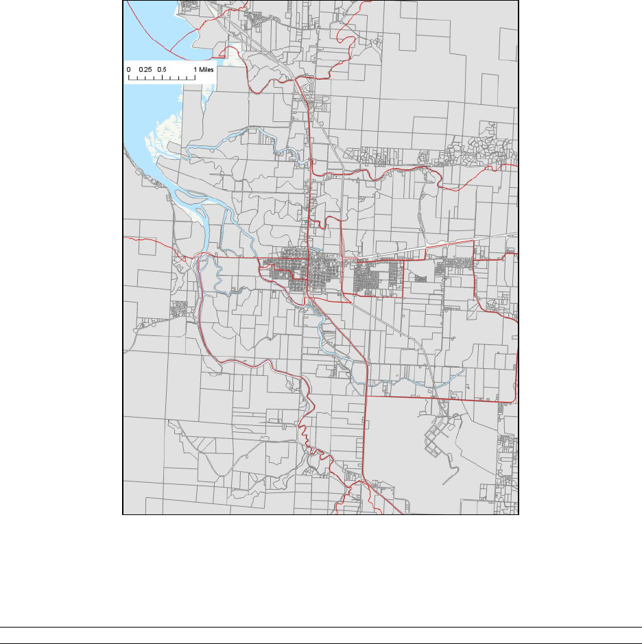
56
A.3 Summary statistics
Table A1. Variable Definitions and Descriptive Statistics, First Analysis Sample, 2009-2017
Variables
Mean
Std Dev
Min
Max
Event
Sold after 2011 Tohoku EQ (tohoku=1)
0.81
(0.39)
0
1
Sold after 2015 article (article=1)
0.33
(0.47)
0
1
Treatment
Inside 1995 SB 379 tsunami zone (sb379=1)
0.27
(0.44)
0
1
Inside 2013 XXL tsunami zone (xxl2013=1)
0.49
(0.50)
0
1
Inside 2013 XL tsunami zone (xl2013=1)
0.47
(0.50)
0
1
Inside 2013 L tsunami zone (l2013=1)
0.34
(0.48)
0
1
Inside 2013 M tsunami zone (m2013=1)
0.25
(0.43)
0
1
Inside 2013 SM tsunami zone (sm2013=1)
0.13
(0.34)
0
1
Structural
Sale price (2019 constant dollars)
311,091.80
(170,179.49)
31,393
1,003,509
Bedrooms
2.83
(0.93)
1
8
Bathrooms
2.02
(0.77)
.5
6
Figure A2. Approximate scale of Census block groups in the city of Tillamook (red).

57
Table A1. Variable Definitions and Descriptive Statistics, First Analysis Sample, 2009-2017
Variables
Mean
Std Dev
Min
Max
Indoor square footage
1,680.60
(705.27)
208
7,265
Total acreage (equal to indoor area if apartment)
0.40
(2.17)
.0057
115
Effective age of property (2018 - remodel year)
36.09
(25.25)
0
137
Heating (=1)
0.94
(0.24)
0
1
Fireplace (=1)
0.65
(0.48)
0
1
Garage (=1)
0.75
(0.43)
0
1
Carport (=1)
0.04
(0.19)
0
1
Deck (=1)
0.12
(0.33)
0
1
Patio (=1)
0.18
(0.38)
0
1
Fencing (=1)
0.15
(0.36)
0
1
Goal 18 eligible (=1)
0.04
(0.19)
0
1
Has shoreline armoring (=1)
0.01
(0.11)
0
1
Location
Special Flood Hazard Area (SFHA) (=1)
0.12
(0.32)
0
1
Elevation (ft)
77.06
(69.47)
0
685
Slope (angular degrees of slope)
2.46
(4.33)
0
32
Distance to nearest beach access point (ft)
3,742.94
(6,488.61)
0
58,260
Distance to ocean shoreline (ft)
13,613.77
(21,683.77)
0
171,886
Oceanfront (=1)
0.05
(0.22)
0
1
Distance to nearest water body (lake, pond, bay) (ft)
6,833.93
(8,262.88)
0
54,308
Distance to nearest river (ft)
7,311.76
(7,987.83)
0
42,105
Distance to nearest state park or public land (ft)
24,815.12
(25,972.40)
0
97,127
Distance to nearest national park or public land (ft)
18,365.10
(17,023.94)
0
74,910
Distance to nearest highway or interstate (ft)
3,164.46
(5,049.39)
0
36,871
Distance to nearest major road (ft)
3,761.70
(6,169.40)
0
36,909
Distance to nearest railroad (ft)
72,756.88
(58,552.91)
21
174,281
Distance to nearest airport (ft)
30,689.69
(19,410.33)
163
83,958
Distance to nearest k-12 school (ft)
14,045.38
(14,543.35)
102
70,987
Distance to nearest central business district (city) (ft)
10,533.27
(10,258.51)
0
71,539
Distance to nearest wastewater treatment plant (ft)
14,574.16
(10,861.35)
44
78,773
Distance to nearest fire station (ft)
6,032.35
(4,741.50)
.85
33,221
Distance to nearest law enforcement station (ft)
31,602.66
(38,338.10)
108
160,319
Distance to nearest hospital (ft)
47,994.08
(43,389.19)
229
167,748
Table A2. Variable Definitions and Descriptive Statistics, Second Analysis Sample, Model 1, 2011-
2015
Variables
Mean
Std Dev
Min
Max
Event
Sold after 2013 map change (after 10/2/13) (newmaps=1)
0.59
(0.49)
0
1
Treatment
Inside 2013 XXL tsunami zone (xxl2013=1)
0.27
(0.44)
0
1
Inside 2013 XL tsunami zone (xl2013=1)
0.24
(0.43)
0
1
Inside 2013 L tsunami zone (l2013=1)
0.11
(0.31)
0
1
Inside 2013 M tsunami zone (m2013=1)
0.04
(0.19)
0
1
Inside 2013 SM tsunami zone (sm2013=1)
0.01
(0.10)
0
1
Structural
Sale price (2019 constant dollars)
296,220.40
(163,439.01)
31,540
1,003,509
Bedrooms
2.87
(0.89)
1
8

58
Table A2. Variable Definitions and Descriptive Statistics, Second Analysis Sample, Model 1, 2011-
2015
Variables
Mean
Std Dev
Min
Max
Bathrooms
2.01
(0.74)
.5
6
Indoor square footage
1,658.07
(714.75)
96
6,577
Total acreage (equal to indoor area if apartment)
0.51
(1.95)
.0023
112
Effective age of property (2018 - remodel year)
35.98
(24.94)
0
137
Heating (=1)
0.77
(0.42)
0
1
Fireplace (=1)
0.57
(0.49)
0
1
Garage (=1)
0.71
(0.45)
0
1
Carport (=1)
0.03
(0.18)
0
1
Deck (=1)
0.09
(0.29)
0
1
Patio (=1)
0.18
(0.38)
0
1
Fencing (=1)
0.12
(0.33)
0
1
Goal 18 eligible (=1)
0.02
(0.13)
0
1
Has shoreline armoring (=1)
0.00
(0.05)
0
1
Location
Special Flood Hazard Area (SFHA) (=1)
0.03
(0.17)
0
1
Elevation (ft)
99.83
(82.15)
0
1,146
Slope (angular degrees of slope)
1.85
(4.26)
0
32
Distance to nearest beach access point (ft)
5,065.92
(8,094.82)
0
74,110
Distance to ocean shoreline (ft)
16,628.09
(20,257.40)
0
137,602
Oceanfront (=1)
0.03
(0.16)
0
1
Distance to nearest water body (lake, pond, bay) (ft)
6,878.71
(7,469.41)
0
60,075
Distance to nearest river (ft)
7,264.15
(7,481.09)
0
42,105
Distance to nearest state park or public land (ft)
23,041.32
(25,780.63)
0
116,124
Distance to nearest national park or public land (ft)
14,391.50
(14,826.84)
0
74,910
Distance to nearest highway or interstate (ft)
3,468.93
(5,347.09)
0
63,013
Distance to nearest major road (ft)
2,805.27
(4,675.05)
0
36,683
Distance to nearest railroad (ft)
85,412.48
(106,850.86)
0
394,958
Distance to nearest airport (ft)
29,597.25
(20,233.50)
474
121,345
Distance to nearest k-12 school (ft)
13,697.00
(15,220.24)
152
99,992
Distance to nearest central business district (city) (ft)
10,798.03
(11,022.24)
0
99,593
Distance to nearest wastewater treatment plant (ft)
16,868.88
(21,145.99)
220
166,371
Distance to nearest fire station (ft)
6,385.07
(5,420.26)
3.4
62,965
Distance to nearest law enforcement station (ft)
25,640.00
(32,459.64)
157
160,319
Distance to nearest hospital (ft)
47,723.01
(48,161.14)
229
176,429
Table A3. Variable Definitions and Descriptive Statistics, by SM2013, Second Analysis Sample,
Model 5, 2011-2015
Outside SM2013 inundation
zone
Inside SM2013 inundation
zone
Mean
Std Dev
Mean
Std Dev
Standardized diff.
in means
Event
Sold after 2013 map change
(after 10/2/13) (newmaps=1)
0.59
(0.49)
0.53
(0.50)
-
Treatment
Inside 2013 XXL tsunami
zone (xxl2013=1)
0.00
(0.00)
1.00
(0.00)
-

59
Table A3. Variable Definitions and Descriptive Statistics, by SM2013, Second Analysis Sample,
Model 5, 2011-2015
Outside SM2013 inundation
zone
Inside SM2013 inundation
zone
Mean
Std Dev
Mean
Std Dev
Standardized diff.
in means
Inside 2013 XL tsunami zone
(xl2013=1)
0.00
(0.00)
1.00
(0.00)
-
Inside 2013 L tsunami zone
(l2013=1)
0.00
(0.00)
1.00
(0.00)
-
Inside 2013 M tsunami zone
(m2013=1)
0.00
(0.00)
1.00
(0.00)
-
Inside 2013 SM tsunami
zone (sm2013=1)
0.00
(0.00)
1.00
(0.00)
-
Structural
Sale price (2019 constant
dollars)
295,066.23
(159,063.84)
231,780.57
(148,962.81)
0.41
Bedrooms
2.90
(0.88)
2.60
(0.96)
0.32
Bathrooms
2.01
(0.75)
1.63
(0.75)
0.51
Indoor square footage
1,675.28
(718.92)
1,400.46
(557.99)
0.43
Total acreage (equal to
indoor area if apartment)
0.45
(1.40)
1.36
(5.21)
-0.24
Effective age of property
(2018 - remodel year)
37.04
(25.55)
40.62
(25.24)
-0.14
Heating (=1)
0.77
(0.42)
0.81
(0.39)
-0.10
Fireplace (=1)
0.58
(0.49)
0.57
(0.50)
0.02
Garage (=1)
0.72
(0.45)
0.74
(0.44)
-0.05
Carport (=1)
0.04
(0.19)
0.01
(0.11)
0.16
Deck (=1)
0.09
(0.28)
0.16
(0.37)
-0.22
Patio (=1)
0.17
(0.38)
0.20
(0.40)
-0.07
Fencing (=1)
0.10
(0.31)
0.15
(0.36)
-0.13
Goal 18 eligible (=1)
0.01
(0.10)
0.06
(0.24)
-0.27
Has shoreline armoring (=1)
0.00
(0.02)
0.02
(0.16)
-0.22
Location
Special Flood Hazard Area
(SFHA) (=1)
0.01
(0.12)
0.33
(0.47)
-0.92
Elevation (ft)
121.66
(86.13)
16.40
(11.41)
1.71
Slope (angular degrees of
slope)
2.04
(4.72)
1.71
(2.68)
0.08
Distance to nearest beach
access point (ft)
5,224.44
(8,615.61)
5,212.64
(8,302.32)
0.00
Distance to ocean shoreline
(ft)
18,437.87
(21,378.82)
24,432.62
(25,851.42)
-0.25
Oceanfront (=1)
0.02
(0.14)
0.14
(0.34)
-0.44

60
Table A3. Variable Definitions and Descriptive Statistics, by SM2013, Second Analysis Sample,
Model 5, 2011-2015
Outside SM2013 inundation
zone
Inside SM2013 inundation
zone
Mean
Std Dev
Mean
Std Dev
Standardized diff.
in means
Distance to nearest water
body (lake, pond, bay) (ft)
6,525.36
(6,387.23)
6,934.80
(7,488.63)
-0.06
Distance to nearest river (ft)
7,041.95
(7,623.14)
2,397.07
(4,759.82)
0.73
Distance to nearest state park
or public land (ft)
21,838.01
(24,637.87)
28,713.47
(42,249.45)
-0.20
Distance to nearest national
park or public land (ft)
12,909.37
(11,189.78)
21,961.15
(20,433.28)
-0.55
Distance to nearest highway
or interstate (ft)
3,062.55
(4,486.45)
2,618.67
(3,738.27)
0.11
Distance to nearest major
road (ft)
2,388.29
(4,137.68)
4,412.83
(4,579.18)
-0.46
Distance to nearest railroad
(ft)
84,464.79
(110,408.42)
91,671.84
(130,852.13)
-0.06
Distance to nearest airport
(ft)
29,363.18
(20,422.74)
29,765.47
(22,999.55)
-0.02
Distance to nearest k-12
school (ft)
12,305.84
(15,174.39)
13,800.28
(17,319.14)
-0.09
Distance to nearest central
business district (city) (ft)
10,406.69
(11,050.82)
12,797.71
(16,355.74)
-0.17
Distance to nearest
wastewater treatment plant
(ft)
15,253.71
(16,461.63)
41,222.65
(57,833.19)
-0.61
Distance to nearest fire
station (ft)
6,106.20
(5,134.15)
6,992.28
(7,554.86)
-0.14
Distance to nearest law
enforcement station (ft)
23,176.83
(30,892.87)
19,219.65
(25,149.62)
0.14
Distance to nearest hospital
(ft)
44,383.06
(48,983.38)
32,092.84
(30,190.89)
0.30
Observations
5348
81
Table A4. Variable Definitions and Descriptive Statistics, by treatment, Third Analysis Sample, Model
62, 2014-2019
Outside blue line
neighborhood (>1000’)
Inside blue line neighborhood
(≤1000’)
Mean
Std Dev
Mean
Std Dev
Standardized
diff. in means
Event
Sold after blue line was
installed (installation=1)
0.15
(0.35)
0.12
(0.33)
-
Structural
Sale price (2019 constant
dollars)
314,429.10
(162,377.00)
309,337.13
(152,322.52)
0.03

61
Table A4. Variable Definitions and Descriptive Statistics, by treatment, Third Analysis Sample, Model
62, 2014-2019
Outside blue line
neighborhood (>1000’)
Inside blue line neighborhood
(≤1000’)
Mean
Std Dev
Mean
Std Dev
Standardized
diff. in means
Bedrooms
2.80
(1.00)
2.73
(0.97)
0.07
Bathrooms
1.97
(0.80)
2.04
(0.83)
-0.09
Indoor square footage
1,430.40
(740.11)
1,516.89
(684.84)
-0.12
Total acreage (equal to
indoor area if apartment)
0.16
(0.28)
0.13
(0.12)
0.10
Effective age of property
(2018 - remodel year)
42.96
(30.13)
44.09
(29.18)
-0.04
Heating (=1)
0.78
(0.42)
0.84
(0.37)
-0.15
Fireplace (=1)
0.60
(0.49)
0.65
(0.48)
-0.10
Garage (=1)
0.61
(0.49)
0.62
(0.49)
-0.01
Carport (=1)
0.05
(0.21)
0.03
(0.17)
0.08
Deck (=1)
0.06
(0.24)
0.08
(0.27)
-0.07
Patio (=1)
0.07
(0.25)
0.05
(0.21)
0.09
Fencing (=1)
0.13
(0.34)
0.11
(0.31)
0.09
Goal 18 eligible (=1)
0.04
(0.19)
0.04
(0.19)
0.00
Has shoreline armoring
(=1)
0.00
(0.07)
0.01
(0.12)
-0.09
Location
Special Flood Hazard
Area (SFHA) (=1)
0.08
(0.27)
0.02
(0.15)
0.25
Elevation (ft)
78.54
(54.42)
72.78
(39.94)
0.12
Slope (angular degrees of
slope)
1.26
(3.22)
1.17
(3.52)
0.03
Distance to nearest beach
access point (ft)
1,753.50
(1,200.59)
1,567.82
(967.45)
0.17
Distance to ocean
shoreline (ft)
7,004.29
(11,446.24)
5,277.00
(9,535.52)
0.16
Oceanfront (=1)
0.05
(0.21)
0.04
(0.20)
0.01
Distance to nearest water
body (lake, pond, bay) (ft)
8,136.05
(10,203.83)
7,562.50
(8,366.73)
0.06
Distance to nearest river
(ft)
8,247.52
(7,645.72)
9,927.78
(7,845.34)
-0.22
Distance to nearest state
park or public land (ft)
39,778.11
(34,629.56)
45,823.91
(35,030.73)
-0.17
Distance to nearest
national park or public
land (ft)
9,977.76
(6,980.00)
11,159.64
(6,648.46)
-0.17
Distance to nearest
2,164.05
(2,831.09)
2,212.84
(2,349.62)
-0.02

62
Table A4. Variable Definitions and Descriptive Statistics, by treatment, Third Analysis Sample, Model
62, 2014-2019
Outside blue line
neighborhood (>1000’)
Inside blue line neighborhood
(≤1000’)
Mean
Std Dev
Mean
Std Dev
Standardized
diff. in means
highway or interstate (ft)
Distance to nearest major
road (ft)
983.77
(1,240.99)
1,076.13
(1,232.81)
-0.07
Distance to nearest
railroad (ft)
102,717.54
(73,404.78)
116,566.90
(79,155.34)
-0.18
Distance to nearest airport
(ft)
36,613.15
(18,433.78)
38,472.42
(18,765.22)
-0.10
Distance to nearest k-12
school (ft)
7,071.64
(7,165.77)
6,593.33
(6,142.44)
0.07
Distance to nearest central
business district (city) (ft)
8,889.72
(6,145.68)
8,469.24
(5,351.54)
0.07
Distance to nearest
wastewater treatment
plant (ft)
15,418.32
(21,860.83)
20,407.66
(28,665.84)
-0.20
Distance to nearest fire
station (ft)
4,308.63
(3,070.37)
4,416.41
(3,412.12)
-0.03
Distance to nearest law
enforcement station (ft)
22,679.32
(39,096.02)
18,610.70
(33,196.20)
0.11
Distance to nearest
hospital (ft)
35,715.25
(50,321.69)
29,175.45
(45,741.74)
0.14
Observations
822
512
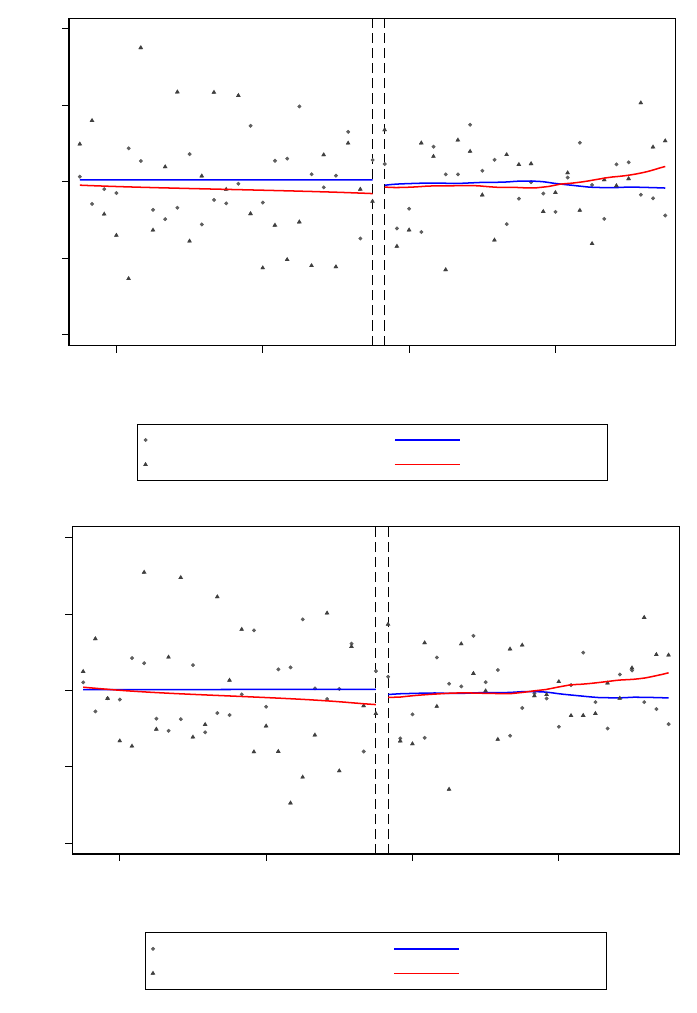
63
A.4 Price trends plots for the second analysis
(a)
(b)
-.2 -.1
0 .1 .2
Residual log sale prices
2012
2013
2014
2015
Year
Control (outside xxl2013) Control trend
Treatment (inside xxl2013) Treatment trend
-.2 -.1 0
.1 .2
Residual log sale prices
2012
2013
2014
2015
Year
Control (outside xl2013) Control trend
Treatment (inside xl2013) Treatment trend
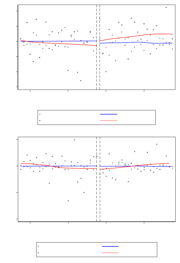
64
(c)
(d)
-.3 -.2 -.1
0 .1 .2
Residual log sale prices
2012
2013
2014
2015
Year
Control (outside l2013) Control trend
Treatment (inside l2013) Treatment trend
2013 map change
-1 -.5 0 .5
Residual log sale prices
2012
2013
2014
2015
Year
Control (outside m2013) Control trend
Treatment (inside m2013) Treatment trend
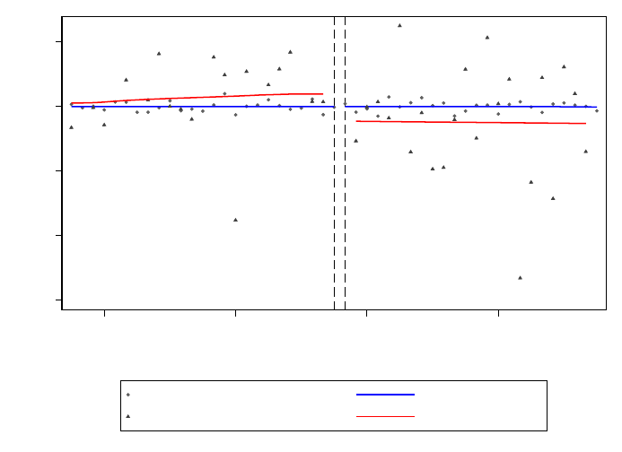
65
(e)
Figure A3.
Housing price trends inside and outside of the treatment inundation line – XXL, Xl, L, M, or SM – for the seven
coastal counties and the second analysis. Plot of residual (log) sale prices net of structural attributes, location covariates, and
fixed effects aggregated by month with local polynomial trend lines. The time range is 2 years before and after the 2013 map
change. Figures (a)-(e) present plots for Models 1-5.
A.5 Tsunami blue line overlap cases
Two binary indicators are needed for the DID and DDD regressions: treatment and event. Treatment defines
whether the transaction is adjacent to a blue line, e.g., inside that blue line’s neighborhood (treatment buffer)
versus not inside the blue line’s neighborhood (control buffer). Event defines whether the transaction occurs
after the blue line was installed. This means that each transaction can fall into one of four categories:
treatment post-installation, treatment pre-installation, control post-installation, and control pre-installation.
For the following explanations we will use the two diagrams below. In both diagrams the small
circular buffer (2000’) determines the treatment buffer and the large circular buffer (4000’) determines the
control buffer. So, the “2017” blue line (blue square) falls in the treatment buffer and the “2018” blue line
falls in the control buffer. The transaction (black point labeled “2016”) falls in both a treatment buffer of
one blue line and a control buffer of another blue line. The diagram on the left is a more intuitive way of
representing what’s happening. The transaction falls in both the treatment and control buffers of the blue
lines but the buffers are centered on the blue lines. This is equivalent to the diagram on the right but not
technically accurate. The diagram on the right is an accurate portrayal of how this is coded in Stata, i.e., the
transaction has distance buffers around it that hold blue lines. For the sake of building intuition, I will use
the diagram on the left to visualize the following overlap cases.
2013 map change
-1.5 -1 -.5 0
.5
Residual log sale prices
2012
2013
2014
2015
Year
Control (outside sm2013)
Control trend
Treatment (inside sm2013) Treatment trend
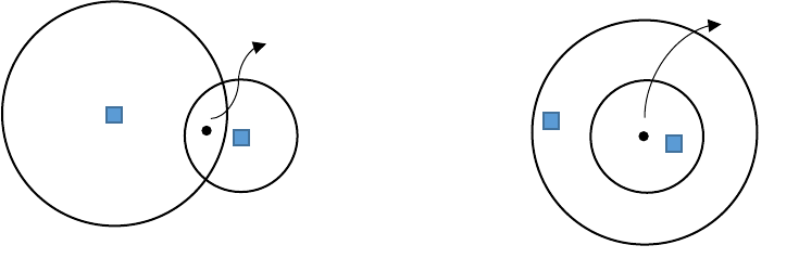
66
The central idea of treatment and event assignment is that “earliest supersedes nearest.” If a
transaction lies within a given buffer distance of two different blue lines and one of the blue lines is installed
before the transaction and the other is installed after the transaction, I use the first-installed blue line as the
reference point, not the nearest blue line. In case there is a tie for earliest because multiple blue lines were
installed at the same time, then the nearest blue line is chosen. Then, I determine whether the transaction
occurred before or after this reference blue line was installed. This is used to create the “event” variable(s).
To create “treatment” variable(s), I tried to consider all possible cases of buffer overlap. The key question
is how should we treat transactions that fall in one blue line’s “treatment” buffer (e.g., 2000’ buffer) and
another blue line’s “control” buffer (e.g., 4000’ buffer)? Which blue line should be chosen as the
appropriate reference point? There are nine total cases that can occur when a treatment buffer and control
buffer overlap for a transaction. I look at 11 cases below but cases 1 and 2 are identical as are cases 3 and
4.
When the transaction occurs between the “treated” and “control” blue line installation dates, timing
matters. In this case, “earliest supersedes nearest” and the first-installed blue line is the reference point.
Cases 5, 6, 8, and 10 apply to this situation. When the transaction occurs before (after) both the “treated”
and “control” blue lines are installed, timing “doesn’t matter” because the transaction is going to be labeled
pre-installation (post-installation) regardless of which blue line is chosen as the reference point. In this case,
distance determines whether the transaction is labeled as a treated or control, i.e., the “earliest supersedes
nearest” principle is not applied in these cases because timing “doesn’t matter.” For example, if the
transaction is in both the treated and control buffer and occurs pre-installation of both blue lines, the
transaction is labeled as treated pre-installation, because the distance to the “treated” blue line is smaller
and because it would be labeled pre-installation regardless. The remaining cases apply to this situation.
2018
2017
2016
4000’
2000’
2018
2017
2016
4000’
2000’
67
Case 1: Treated pre-installation and control pre-installation: the
transaction is in the treated buffer before the blue line’s installation and
in the control buffer before the blue line’s installation. Timing “doesn’t
matter” here because the transaction occurs before both the “treated”
and “control” blue lines are installed. Since timing doesn’t matter,
distance determines whether it’s treated or control. In this case, since
it’s in both, it’s treated. So, the transaction should be used as treated
pre-installation.
Case 2: Treated pre-installation and control pre-installation. The
transaction should be used as treated pre-installation as in case 1.
Case 3: Treated post-installation and control post-installation. Timing
“doesn’t matter” here because the transaction occurs after both the
“treated” and “control” blue lines are installed. Since timing doesn’t
matter, distance determines whether it’s treated or control. In this case,
since it’s in both, it’s treated. So, the transaction should be used as
treated post-installation.
Case 4: Treated post-installation and control post-installation. The
transaction should be used as treated pre-installation as in case 3.
2018
2017
2016
4000
2000
2017
2018
2016
4000
2000
2018
2017
2019
4000
2000
2017
2018
2019
4000
2000
68
Case 5: Treated post-installation and control pre-installation. Now
timing matters because the transaction occurs between the installation
of the blue line whose control group it’s in and the blue line whose
treatment group it’s in. “Earliest supersedes nearest” means that it’s
the blue line that’s installed first that the event and treatment decision
should be based on. So, since the transaction is post-installation of the
treatment blue line, it should be used as treated post-installation.
Case 6: Treated pre-installation and control post-installation. Timing
matters because the transaction occurs between the installation of the
blue line whose control group it’s in and the blue line whose treatment
group it’s in. “Earliest supersedes nearest” means that it’s the blue line
that’s installed first that the event and treatment decision should be
based on. So, since the transaction is post-installation of the control
blue line, it should be used as control post-installation.
Case 7: Treated pre-installation and control is at installation (the
transaction date and installation date of the blue line defining the
control buffer is the same). When the transaction date is at the same
time as the blue line installation date this is considered to be “pre-
installation” because the blue line hasn’t been in place long enough to
affect the sale price of the property being sold at the same time. So,
this is technically a “control pre-installation” situation. Thus, this is like case 2 and the transaction should
be used as treated pre-installation.
Case 8: Treated post-installation and control is at installation (the
transaction date and installation date of the blue line defining the
control buffer is the same). For the same reasons as in case 7, this is
technically a “control pre-installation” situation. Thus, this is like case
5 and the transaction should be used as treated post-installation.
2018
2016
2017
4000
2000
2016
2018
2017
4000
2000
2017
2018
2017
4000
2000
2017
2016
2017
4000
2000
69
Case 9: Control pre-installation and treated is at installation (the
transaction date and installation date of the blue line defining the
treatment buffer is the same). For the same reasons as in case 7, this is
technically a “treatment pre-installation” situation. Thus, this is like
case 1 and the transaction should be used as treated pre-installation.
Case 10: Control post-installation and treated is at installation (the
transaction date and installation date of the blue line defining the
treatment buffer is the same). For the same reasons as in case 7, this is
technically a “treatment pre-installation” situation. Thus, this is like
case 6 and the transaction should be used as control post-installation.
Case 11: Treated and control are at installation (the transaction date
and installation dates of both blue lines are all the same). For the same
reasons as in case 7, this is technically a “treatment pre-installation”
and “control pre-installation” situation. Thus, this is like case 1 and the
transaction should be used as a treated pre-installation.
A.6 Matching results for the first analysis
Tables A5, A6, A7, and A8 report the covariate balance results for the PSM, NNM, CEM and EB
matching/weighting methods, respectively. The standardized difference in means for the variables used in
each procedure is measured for all the primary models before matching/weighting (raw) and after
matching/weighting (matched/weighted). The PSM method (Table A5) improved covariate balance for the
key variables that likely influence treatment – elevation and distance to the ocean – in all models. However,
the absolute standardized difference in means for the elevation variable in Model III did not decrease to
below 0.25, the aforementioned rule of thumb indicating covariate balance (Stuart, 2010). Furthermore,
approximately 87-92% of the control observations are dropped after matching, depending on the model. An
additional drawback of propensity score matching was the inability to exactly match on event timing. The
NNM method (Table A6) also improved covariate balance for the key matching variables but still did not
achieve covariate balance according to the rule of thumb for the elevation variable in Models I and III.
2018
2017
2017
4000
2000
2016
2017
2017
4000
2000
2017
2017
2017
4000
2000

70
Unlike PSM, NNM was able to exactly match on the events of interest. Similar to PSM, however, NNM
dropped approximately 89-93% of the control observations. The CEM method (Table A7) did not
appreciably improve covariate balance.
35
The absolute standardized difference in means for elevation and
distance to the ocean did not decrease to below the rule of thumb. However, the CEM method does not drop
90% of control observations, unlike the PSM and NNM methods. The EB method (Table A8) improved
covariate balance for the key matching variables but did not achieve covariate balance according to the rule
of thumb for the elevation variable in Models I and III.
36
Unlike the other three methods, however, the EB
method is purely a weighting method and, as such, does not drop observations. However, an inspection of
the weights generated by EB shows that many observations are assigned very small weights, suggesting
that this method also effectively “drops” many control observations. In summary, the two matching
methods (PSM and NNM) that improved covariate balance for the key variables that likely influence
treatment also dropped approximately 90% of the control observations and the matching method (CEM)
that does not drop most of the control observations also does not appreciably improve covariate balance.
Table A5. Propensity score matching standardized differences for the first analysis
Model I
Model II
Model III
Variables
Raw
Matched
Raw
Matched
Raw
Matched
Sold after 2011 Tohoku EQ (tohoku=1)
0.0463
-0.0038
0.0136
0.1306
Sold after 2015 article (article=1)
-0.0097
0.0041
-0.0032
-0.0067
Elevation (ft)
-1.5211
-0.1239
-1.7165
-0.1151
-1.5148
-0.2765
Log distance to ocean shoreline
-0.6606
0.0708
-0.7227
0.1190
-0.6743
0.1865
Sale year of the property
0.0368
0.0280
-0.0055
0.1225
0.0017
0.1181
Observations
5,890
1,932
9,160
4,996
15,627
5,088
Treatment
1,589
1,589
4,471
4,384
4,160
4,160
Control
4,301
343
4,689
612
11,467
928
Table A6. Nearest neighbor Mahalanobis matching standardized differences for the first analysis
Model I
Model II
Model III
Variables
Raw
Matched
Raw
Matched
Raw
Matched
Elevation (ft)
-1.5211
-0.3381
-1.7209
-0.0966
-1.5148
-0.3211
Log distance to ocean shoreline
-0.6606
-0.0218
-0.7361
-0.0315
-0.6743
-0.0205
Sale year of the property
0.0368
-0.0042
-0.0037
-0.0078
0.0017
0.0007
Observations
5,890
1,902
9,160
4,983
15,627
4,980
Treatment
1,589
1,589
4,471
4,471
4,160
4,160
Control
4,301
313
4,689
512
11,467
820
35
Table A7 reports unweighted standardized differences. Future iterations of this paper will report weighted standardized
differences since CEM is a weighting method and therefore drops few observations.
36
Table A8 reports unweighted standardized differences. Future iterations of this paper will report weighted standardized
differences since EB is a weighting method and therefore drops few observations.

71
Table A6. Nearest neighbor Mahalanobis matching standardized differences for the first analysis
Model I
Model II
Model III
Variables
Raw
Matched
Raw
Matched
Raw
Matched
Exact matching on event (tohoku and/or article).
Table A7. Coarsened exact matching standardized differences for the first analysis
Model I
Model II
Model III
Variables
Raw
Matched
Raw
Matched
Raw
Matched
Sold after 2011 Tohoku EQ (tohoku=1)
-0.0463
-0.0738
-0.0136
0.0105
Sold after 2015 article (article=1)
0.0079
-0.0567
0.0032
-0.0211
Elevation (ft)
1.5211
1.2699
1.7209
1.1031
1.5148
1.2832
Log distance to ocean shoreline
0.6606
0.4441
0.7361
0.5445
0.6743
0.3887
Sale year of the property
-0.0368
-0.0640
0.0037
-0.0421
-0.0017
0.0081
Observations
5,890
3,447
9,160
5,771
15,627
9,202
Treatment
1,589
1,540
4,471
4,188
4,160
3,987
Control
4,301
1,907
4,689
1,583
11,467
5,215
Table A8. Entropy balancing standardized differences for the first analysis
Model I
Model II
Model III
Variables
Raw
Weighted
Raw
Weighted
Raw
Weighted
Sold after 2011 Tohoku EQ (tohoku=1)
0.0463
-0.0013
0.0136
-0.0006
Sold after 2015 article (article=1)
-0.0079
-0.0005
-0.0032
-0.0028
Elevation (ft)
-1.5211
-0.2852
-1.7209
-0.1697
-1.5148
-0.2699
Log distance to ocean shoreline
-0.6606
0.0042
-0.7361
-0.0021
-0.6743
0.0006
Sale year of the property
0.0368
-0.0005
-0.0037
0.0001
0.0017
-0.0005
A.7 Regression results and figures
Table A9. Difference-in-differences results for the first analysis, full data
Model I
Model II
Model III
Variables
Coefficient/SE
Coefficient/SE
Coefficient/SE
Event
Sold after 2011 Tohoku EQ (tohoku=1)
.0858**
.0631
(.0426)
(.0390)
Sold after 2015 article (article=1)
.0136
.0026
(.0236)
(.0200)
Treatment
Inside 1995 SB 379 tsunami zone (sb379=1)
.0620*
.0671**
(.0333)
(.0308)
Inside 2013 XXL tsunami zone (xxl2013=1)
-.0073
(.0222)
Diff-in-Diff
SB 379 zone (sb379) x sold after 2011 Tohoku EQ (tohoku)
-.0889**
-.0675**
(.0415)
(.0340)

72
Table A9. Difference-in-differences results for the first analysis, full data
Model I
Model II
Model III
Variables
Coefficient/SE
Coefficient/SE
Coefficient/SE
2013 XXL zone (xxl2013) x sold after 2015 article (article)
.0064
(.0240)
SB 379 zone (sb379) x sold after 2015 article (article)
.0269
(.0244)
Structural
Bedrooms
.1115***
.0323
.0592***
(.0337)
(.0233)
(.0191)
Bedrooms squared
-.0189***
-.0083**
-.0117***
(.0051)
(.0035)
(.0029)
Bathrooms
.1278***
.1688***
.1576***
(.0403)
(.0344)
(.0253)
Bathrooms squared
-.0094
-.0184**
-.0165***
(.0082)
(.0075)
(.0054)
Indoor square footage
3.7e-04***
5.0e-04***
4.5e-04***
(4.5e-05)
(3.3e-05)
(2.7e-05)
Indoor square footage squared
-4.0e-08***
-5.5e-08***
-4.9e-08***
(9.5e-09)
(7.1e-09)
(5.7e-09)
Total acreage (equal to indoor area if apartment)
.0160*
.0409***
.0274***
(.0095)
(.0068)
(.0048)
Total acreage squared
-2.5e-05
-4.4e-04***
-1.4e-04***
(8.8e-05)
(9.9e-05)
(5.3e-05)
Effective age of property (2018 - remodel year)
.0121***
.0105***
.0113***
(.0012)
(9.1e-04)
(7.1e-04)
Effective age of property squared
-1.4e-04***
-1.3e-04***
-1.3e-04***
(1.2e-05)
(8.8e-06)
(6.9e-06)
Heating (=1)
.1378***
.2823***
.2391***
(.0374)
(.0255)
(.0208)
Fireplace (=1)
.1208***
.0877***
.1009***
(.0171)
(.0120)
(.0097)
Garage (=1)
.0923***
.0510***
.0651***
(.0186)
(.0132)
(.0105)
Goal 18 eligible (=1)
.0860
.0847**
.0788**
(.0576)
(.0400)
(.0326)
Location
Special Flood Hazard Area (SFHA) (=1)
-.0448
-.0377*
-.0397**
(.0275)
(.0193)
(.0159)
Elevation (ft)
5.7e-04***
2.6e-04**
4.6e-04***
(1.7e-04)
(1.3e-04)
(9.8e-05)
Log distance to nearest beach access point
-.0239**
-.0280***
-.0269***
(.0093)
(.0057)
(.0050)
Log distance to ocean shoreline
-.0835***
-.0746***
-.0786***
(.0115)
(.0059)
(.0055)
Elevation (ft) x Log distance to ocean shoreline x on
oceanfront (=1)
3.9e-04***
2.7e-04***
3.2e-04***
(7.7e-05)
(7.4e-05)
(5.3e-05)
Log distance to nearest river
-.0191***
-.0211***
-.0214***
(.0056)
(.0039)
(.0032)
Log distance to nearest national park or public land
-.0374***
-.0336***
-.0344***
(.0098)
(.0057)
(.0050)
Log distance to nearest highway or interstate
.0233***
.0137**
.0160***
(.0077)
(.0054)
(.0044)
Log distance to nearest railroad
-.0185
-.0403***
-.0269***

73
Table A9. Difference-in-differences results for the first analysis, full data
Model I
Model II
Model III
Variables
Coefficient/SE
Coefficient/SE
Coefficient/SE
(.0167)
(.0117)
(.0100)
Log distance to nearest airport
.0434*
.0213
.03066**
(.0223)
(.0160)
(.0128)
Log distance to nearest k-12 school
.0264*
.0305***
.0244***
(.0149)
(.0104)
(.0084)
Log distance to nearest wastewater treatment plant
-.0230
-.0286***
-.0255***
(.0145)
(.0107)
(.0085)
Log distance to nearest hospital
.0409
.0681***
.0587***
(.0260)
(.0177)
(.0144)
Observations
5890
9160
15627
Adj. R-squared
0.376
0.441
0.411
* p<0.10, ** p<0.05, *** p<0.01
Table A10. DID falsification test results for the first analysis, full data
Model I
Model II
Model III
Coefficient/SE
Coefficient/SE
Coefficient/SE
Test #1
SB 379 zone (sb379) x sold after 3/11/10 (falsetohoku)
-.0547
-.0507
(.0463)
(.0431)
SB 379 zone (sb379) x sold after 2015 article (article)
.0169
(.0237)
Test #2
SB 379 zone (sb379) x sold after 3/11/12 (falsetohoku)
-.0153
-.0092
(.0442)
(.0299)
SB 379 zone (sb379) x sold after 2015 article (article)
.0142
(.0252)
Test #3
Placebo treatment group (randomtreat) x sold after 2011
Tohoku EQ (tohoku)
.0199
.0211
(.0270)
(.0216)
Placebo treatment group (randomtreat) x sold after 2015
article (article)
-.0134
5.1e-04
(.0196)
(.0169)
Test #4
SB 379 zone (sb379) x placebo event status (randomevent)
-.0154
(.0306)
2013 XXL zone (xxl2013) x placebo event status
(randomevent)
.0044
(.0193)
* p<0.10, ** p<0.05, *** p<0.01
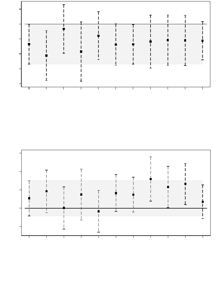
74
(a)
(b)
Figure A4. Average treatment effect on the treated estimates with 95% confidence intervals for the first analysis’ models.
The full data estimator is on the left. The next four points represent the estimators after the data was processed with the four
matching methods (PSM, NNM, CEM, and EB). OB represents the Oaxaca-Blinder estimator. The final six estimators represent
the full data estimator under different sample space assumptions. (a) For Model III’s Tohoku event estimator. (b) For Model
III’s article event estimator.
-.2 -.15
-.1 -.05 0 .05
Coefficients: sb379xtohoku
Full
PSM
NNM
CEM
EB
Full - 1/2 mile
Full - 2 miles
Full - 1/2 mile, 1 year
Full - 1 mile, 1 year
Full - 2 miles, 1 year
Full - 7 counties
Model
y
-.05 0 .05
.1 .15
Coefficients: sb379xarticle
Full
PSM
NNM
CEM
EB
Full - 1/2 mile
Full - 2 miles
Full - 1/2 mile, 1 year
Full - 1 mile, 1 year
Full - 2 miles, 1 year
Full - 7 counties
Model
y

75
Table A11. Difference-in-differences results for the second analysis, full data
Model 1
Model 2
Model 3
Model 4
Model 5
Variables
Coefficient/SE
Coefficient/SE
Coefficient/SE
Coefficient/SE
Coefficient/SE
Event
Sold after 2013 map
change (after 10/2/13)
(newmaps=1)
.0073
.0015
-.0227
-.0176
-.0082
(.0361)
(.0365)
(.0394)
(.0420)
(.0438)
Treatment
Inside 2013 XXL tsunami
zone (xxl2013=1)
-.0145
(.0260)
Inside 2013 XL tsunami
zone (xl2013=1)
-4.6e-04
(.0277)
Inside 2013 L tsunami
zone (l2013=1)
.0073
(.0399)
Inside 2013 M tsunami
zone (m2013=1)
.0434
(.0624)
Inside 2013 SM tsunami
zone (sm2013=1)
.1460
(.1151)
Diff-in-Diff
2013 XXL zone
(xxl2013) x sold after
2013 map change
(newmaps)
.0201
(.0313)
2013 XL zone (xl2013) x
sold after 2013 map
change (newmaps)
.0198
(.0331)
2013 L zone (l2013) x
sold after 2013 map
change (newmaps)
.0710
(.0468)
2013 M zone (m2013) x
sold after 2013 map
change (newmaps)
-.0212
(.0777)
2013 SM zone (sm2013)
x sold after 2013 map
change (newmaps)
-.3097**
(.1502)
Structural
Bedrooms
.0608**
.0581**
.0592**
.0734**
.0724**
(.0247)
(.0250)
(.0264)
(.0291)
(.0296)
Bedrooms squared
-.0096***
-.0091**
-.0097***
-.0116***
-.0114***
(.0035)
(.0035)
(.0037)
(.0042)
(.0042)
Bathrooms
.2820***
.2728***
.2639***
.2723***
.2505***
(.0363)
(.0369)
(.0400)
(.0430)
(.0425)
Bathrooms squared
-.0356***
-.0334***
-.0309***
-.0324***
-.0277***
(.0077)
(.0078)
(.0084)
(.0090)
(.0086)

76
Table A11. Difference-in-differences results for the second analysis, full data
Model 1
Model 2
Model 3
Model 4
Model 5
Variables
Coefficient/SE
Coefficient/SE
Coefficient/SE
Coefficient/SE
Coefficient/SE
Indoor square footage
2.8e-04***
2.9e-04***
3.0e-04***
3.2e-04***
3.3e-04***
(3.5e-05)
(3.6e-05)
(3.9e-05)
(4.1e-05)
(4.4e-05)
Indoor square footage
squared
-1.8e-08**
-2.1e-08***
-2.3e-08***
-2.5e-08***
-2.9e-08***
(7.3e-09)
(7.4e-09)
(7.9e-09)
(8.3e-09)
(8.8e-09)
Total acreage (equal to
indoor area if apartment)
.0354***
.0393***
.0375***
.0346***
.0697***
(.0080)
(.0081)
(.0098)
(.0101)
(.0116)
Total acreage squared
-2.7e-04***
-3.0e-04***
-2.7e-04***
-2.3e-04***
-.0016***
(8.0e-05)
(7.8e-05)
(8.4e-05)
(8.8e-05)
(.0005)
Effective age of property
(2018 - remodel year)
.0099***
.0100***
.0098***
.0105***
.0105***
(.001)
(.0010)
(.00112)
(.0012)
(.0013)
Effective age of property
squared
-1.2e-04***
-1.2e-04***
-1.2e-04***
-1.3e-04***
-1.3e-04***
(9.6e-06)
(9.7e-06)
(1.1e-05)
(1.1e-05)
(1.2e-05)
Heating (=1)
.1953***
.2145***
.2087***
.2352***
.2351***
(.0321)
(.0321)
(.0343)
(.0383)
(.0389)
Fireplace (=1)
.1009***
.0956***
.0925***
.0713***
.0771***
(.0142)
(.0144)
(.0155)
(.0163)
(.0168)
Garage (=1)
.0858***
.0787***
.0642***
.0697***
.0669***
(.0150)
(.0152)
(.0165)
(.0177)
(.0185)
Carport (=1)
-.0700**
-.0744**
-.0925***
-.0806**
-.0845**
(.0301)
(.0305)
(.0349)
(.0377)
(.0380)
Deck (=1)
-.0091
-.0114
-.0026
-.0043
.0051
(.0218)
(.0219)
(.0243)
(.0261)
(.0268)
Patio (=1)
.0213
.0184
.0208
.0157
.0299
(.0159)
(.0162)
(.0177)
(.0190)
(.0194)
Fencing (=1)
.0147
.0168
.0217
.0130
.0098
(.0194)
(.0196)
(.0212)
(.0233)
(.0239)
Goal 18 eligible (=1)
.0883
.0892
.1473**
.1219
.0909
(.0641)
(.0652)
(.0722)
(.0829)
(.0884)
Has shoreline armoring
(=1)
.3457***
.3900***
.2800***
.2801**
.3175**
(.0853)
(.0836)
(.0955)
(.1360)
(.1447)
Location
Special Flood Hazard
Area (SFHA) (=1)
-.0131
-.0120
-.0542
-.0227
.0403
(.0395)
(.0405)
(.0454)
(.0573)
(.0591)
Elevation (ft)
6.4e-04***
6.7e-04***
6.9e-04***
6.5e-04***
5.8e-04***
(1.1e-04)
(1.1e-04)
(1.1e-04)
(1.2e-04)
(1.2e-04)
Elevation (ft) x Log
distance to ocean
shoreline x on oceanfront
(=1)
2.0e-04***
1.9e-04***
2.1e-04***
2.1e-04***
1.8e-04***
(6.9e-05)
(7.0e-05)
(6.7e-05)
(6.2e-05)
(6.3e-05)
Slope (angular degrees of
slope)
-.0035
-.0020
-.0019
4.2e-04
.0014
(.0027)
(.0027)
(.0028)
(.0030)
(.0030)
Log distance to nearest
beach access point
-.0157*
-.0132
-.0237***
-.0163*
-.0040
(.0080)
(.0080)
(.0090)
(.0098)
(.0110)

77
Table A11. Difference-in-differences results for the second analysis, full data
Model 1
Model 2
Model 3
Model 4
Model 5
Variables
Coefficient/SE
Coefficient/SE
Coefficient/SE
Coefficient/SE
Coefficient/SE
Log distance to ocean
shoreline
-.1102***
-.1067***
-.0913***
-.0998***
-.1239***
(.0140)
(.0142)
(.0163)
(.0180)
(.0161)
Log distance to nearest
water body (lake, pond,
bay)
-.0030
-.0050
.0011
-4.1e-04
.0064
(.0067)
(.0066)
(.0084)
(.0101)
(.0123)
Log distance to nearest
river
-.0350***
-.0338***
-.0322***
-.0285***
-.0249***
(.0056)
(.0057)
(.0068)
(.0083)
(.0095)
Log distance to nearest
state park or public land
.0029
.0045
2.2e-06
.0100
.0210*
(.0067)
(.0068)
(.0072)
(.0099)
(.0114)
Log distance to nearest
national park or public
land
-.0095
-.0064
-.0060
-.0131
-.0157*
(.0073)
(.0077)
(.0085)
(.0089)
(.0089)
Log distance to nearest
highway or interstate
.0253***
.0241***
.03085***
.0307***
.0288***
(.0090)
(.0061)
(.0069)
(.0078)
(.0083)
Log distance to nearest
major road
4.8e-04
9.8e-04
.0061
.0062
.0070
(.0043)
(.0043)
(.0048)
(.0054)
(.0057)
Log distance to nearest
railroad
-.0090
-.0046
-.0109
-.0122
-.0141
(.0144)
(.0144)
(.0142)
(.0158)
(.0193)
Log distance to nearest
airport
.0410*
.0388*
.0443*
.0183
-.0030
(.0214)
(.0217)
(.0237)
(.0258)
(.0279)
Log distance to nearest k-
12 school
.0052
.0059
.0095
.0257*
.0242*
(.0121)
(.0122)
(.0131)
(.0139)
(.0147)
Log distance to nearest
central business district
(city)
.0188*
.0160
.0156
.0130
.0086
(.0109)
(.0110)
(.0121)
(.0129)
(.0137)
Log distance to nearest
wastewater treatment
plant
-.0191
-.0245*
-.0304*
-.0458***
-.0591***
(.0136)
(.0138)
(.0159)
(.0172)
(.0184)
Log distance to nearest
fire station
-1.2e-04
.0025
.0060
.0005
.0049
(.0106)
(.0108)
(.0126)
(.0146)
(.0151)
Log distance to nearest
law enforcement station
.0106
.0101
.0076
.0144
.0129
(.0141)
(.0143)
(.0155)
(.0168)
(.0175)
Log distance to nearest
hospital
-.01560
-.0207
-.0101
-.0222
-.0392
(.0183)
(.0187)
(.0209)
(.0234)
(.0249)
Observations
8010
7790
6593
5842
5429
Adj. R-squared
0.421
0.420
0.424
0.423
0.427

78
Table A11. Difference-in-differences results for the second analysis, full data
Model 1
Model 2
Model 3
Model 4
Model 5
Variables
Coefficient/SE
Coefficient/SE
Coefficient/SE
Coefficient/SE
Coefficient/SE
* p<0.10, ** p<0.05, *** p<0.01
Table A12. Difference-in-differences results for the second analysis, combined model, full data
Coefficient
SE
Event
Sold after 2013 map change (after 10/2/13) (newmaps=1)
.0077
(.0360)
Treatment
Inside 2013 XXL tsunami zone (xxl2013=1)
-.0491
(.0541)
Inside 2013 XL tsunami zone (xl2013=1)
.0284
(.0582)
Inside 2013 L tsunami zone (l2013=1)
-.0047
(.0495)
Inside 2013 M tsunami zone (m2013=1)
.0144
(.0738)
Inside 2013 SM tsunami zone (sm2013=1)
.0562
(.0964)
Diff-in-Diff
2013 XXL zone (xxl2013) x sold after 2013 map change (newmaps)
-.0477
(.0728)
2013 XL zone (xl2013) x sold after 2013 map change (newmaps)
.0559
(.0778)
2013 L zone (l2013) x sold after 2013 map change (newmaps)
.0903
(.0575)
2013 M zone (m2013) x sold after 2013 map change (newmaps)
-.0556
(.0890)
2013 SM zone (sm2013) x sold after 2013 map change (newmaps)
-.2393*
(.1343)
Structural
Bedrooms
.0617**
(.0246)
Bedrooms squared
-.0097***
(.0035)
Bathrooms
.2796***
(.0363)
Bathrooms squared
-.0349***
(.0077)
Indoor square footage
2.8e-04***
(3.6e-05)
Indoor square footage squared
-1.9e-08**
(7.3e-09)
Total acreage (equal to indoor area if apartment)
.0365***
(.0081)
Total acreage squared
-2.8e-04***
(8.0e-05)
Effective age of property (2018 - remodel year)
.0098***
(.0010)
Effective age of property squared
-1.2e-04***
(9.6e-06)
Heating (=1)
.1949***
(.0321)
Fireplace (=1)
.1009***
(.0143)
Garage (=1)
.0871***
(.0149)
Carport (=1)
-.0699**
(.0302)
Deck (=1)
-.0098
(.0218)
Patio (=1)
.0220
(.0159)
Fencing (=1)
.0153
(.0193)
Goal 18 eligible (=1)
.0910
(.0638)
Has shoreline armoring (=1)
.3085***
(.0838)
Location
Distance (ft) to 2013 XXL line if inside zone (=0 if outside of zone)
2.7e-05
(2.1e-05)
Special Flood Hazard Area (SFHA) (=1)
-.0134
(.0393)
Elevation (ft)
6.6e-04***
(1.1e-04)
Slope (angular degrees of slope)
-.0028
(.0026)
Log distance to nearest beach access point
-.0135*
(.0080)
Log distance to ocean shoreline
-.1096***
(.0140)
Elevation (ft) x Log distance to ocean shoreline x on oceanfront (=1)
2.0e-04***
(7.0e-05)
Log distance to nearest water body (lake, pond, bay)
-.0029
(.0067)
Log distance to nearest river
-.0348***
(.0056)
Log distance to nearest state park or public land
.0032
(.0067)

79
Table A12. Difference-in-differences results for the second analysis, combined model, full data
Coefficient
SE
Log distance to nearest national park or public land
-.0091
(.0073)
Log distance to nearest highway or interstate
.0238***
(.0060)
Log distance to nearest major road
-1.0e-04
(.0043)
Log distance to nearest railroad
-.0067
(.0144)
Log distance to nearest airport
.0408*
(.0214)
Log distance to nearest k-12 school
.0028
(.0121)
Log distance to nearest central business district (city)
.0168
(.0110)
Log distance to nearest wastewater treatment plant
-.0197
(.0136)
Log distance to nearest fire station
.0018
(.0106)
Log distance to nearest law enforcement station
.0134
(.0141)
Log distance to nearest hospital
-.0175
(.0183)
Observations
8010
Adj. R-squared
0.423
* p<0.10, ** p<0.05, *** p<0.01
Table A13. Oaxaca-Blinder results for the second analysis, full data
Model 1
Model 2
Model 3
Model 4
Model 5
Coefficient/SE
Coefficient/SE
Coefficient/SE
Coefficient/SE
Coefficient/SE
Overall Differential
Treated group
12.470***
12.484***
12.514***
12.374***
12.219***
(.0178)
(.0188)
(.0276)
(.0509)
(.0985)
Control group
12.431***
12.435***
12.437***
12.439***
12.437***
(.0073)
(.0073)
(.0076)
(.0079)
(.0081)
Difference
.0390**
.0500**
.0771***
-.0650
-.2184**
(.0193)
(.0202)
(.0287)
(.0515)
(.0988)
Decomposition
Explained
.0094
.0149
.0233
-.0247
-.0466
(.0242)
(.0255)
(.0360)
(.0590)
(.1103)
Unexplained
.0296
.0350
.0539
-.0403
-.1718
(.0249)
(.0261)
(.0357)
(.0597)
(.1047)
Observations
8010
7790
6593
5842
5429
* p<0.10, ** p<0.05, *** p<0.01
Table A14. DID falsification test results for the second analysis, full data
Model 1
Model 2
Model 3
Model 4
Model 5
Coefficient/SE
Coefficient/SE
Coefficient/SE
Coefficient/SE
Coefficient/SE
Test #1
2013 XXL zone
(xxl2013) x sold after
10/2/12 (falsenewmaps)
-.0667*
(.0364)
2013 XL zone (xl2013) x
sold after 10/2/12
(falsenewmaps)
-.0728*
(.0393)
2013 L zone (l2013) x
-.0151

80
Table A14. DID falsification test results for the second analysis, full data
Model 1
Model 2
Model 3
Model 4
Model 5
Coefficient/SE
Coefficient/SE
Coefficient/SE
Coefficient/SE
Coefficient/SE
sold after 10/2/12
(falsenewmaps)
(.0555)
2013 M zone (m2013) x
sold after 10/2/12
(falsenewmaps)
-.0909
(.0809)
2013 SM zone (sm2013)
x sold after 10/2/12
(falsenewmaps)
-.0871
(.1569)
Test #2
2013 XXL zone
(xxl2013) x sold after
10/2/14 (falsenewmaps)
.0288
(.0304)
2013 XL zone (xl2013) x
sold after 10/2/14
(falsenewmaps)
.0370
(.0313)
2013 L zone (l2013) x
sold after 10/2/14
(falsenewmaps)
.0889**
(.0432)
2013 M zone (m2013) x
sold after 10/2/14
(falsenewmaps)
.0627
(.0766)
2013 SM zone (sm2013)
x sold after 10/2/14
(falsenewmaps)
-.1252
(.1559)
Test #3
Placebo treatment group
(randomtreat) x sold after
2013 map change
(newmaps)
-.0197
.0197
.0132
.0419
.0052
(.0229)
(.0230)
(.0253)
(.0269)
(.0281)
Test #4
2013 XXL zone
(xxl2013) x placebo event
status (randomevent)
.0248
(.0251)
2013 XL zone (xl2013) x
placebo event status
(randomevent)
.0300
(.0266)
2013 L zone (l2013) x
placebo event status
(randomevent)
-.0025
(.0361)
2013 M zone (m2013) x
.0118
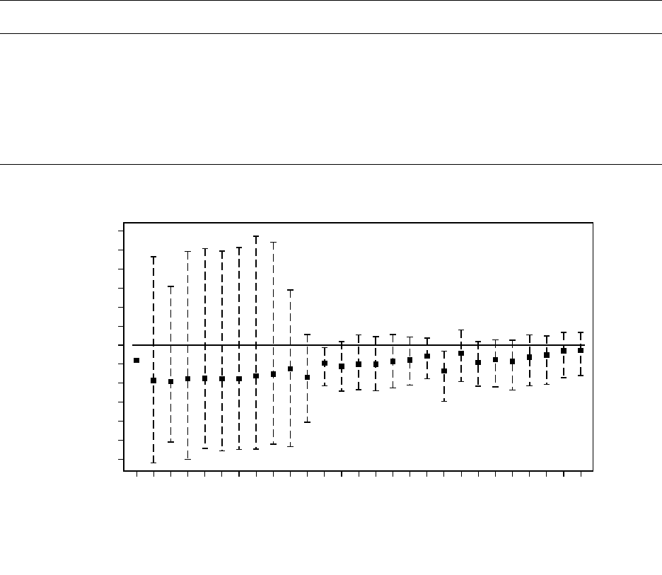
81
Table A14. DID falsification test results for the second analysis, full data
Model 1
Model 2
Model 3
Model 4
Model 5
Coefficient/SE
Coefficient/SE
Coefficient/SE
Coefficient/SE
Coefficient/SE
placebo event status
(randomevent)
(.0647)
2013 SM zone (sm2013)
x placebo event status
(randomevent)
.1576
(.1298)
* p<0.10, ** p<0.05, *** p<0.01
(a)
-.6 -.5 -.4 -.3
-.2 -.1 0 .1 .2 .3
.4 .5 .6
Coefficients
1 - 500, 1000
2 - 500, 1500
3 - 500, 2000
4 - 500, 2500
5 - 500, 3000
6 - 500, 3500
7 - 500, 4000
8 - 500, 4500
9 - 500, 5000
10 - 1000, 1500
11 - 1000, 2000
12 - 1000, 2500
13 - 1000, 3000
14 - 1000, 3500
15 - 1000, 4000
16 - 1000, 4500
17 - 1000, 5000
18 - 1000, 5500
19 - 1500, 2000
20 - 1500, 2500
21 - 1500, 3000
22 - 1500, 3500
23 - 1500, 4000
24 - 1500, 4500
25 - 1500, 5000
26 - 1500, 5500
27 - 1500, 6000
y ( )
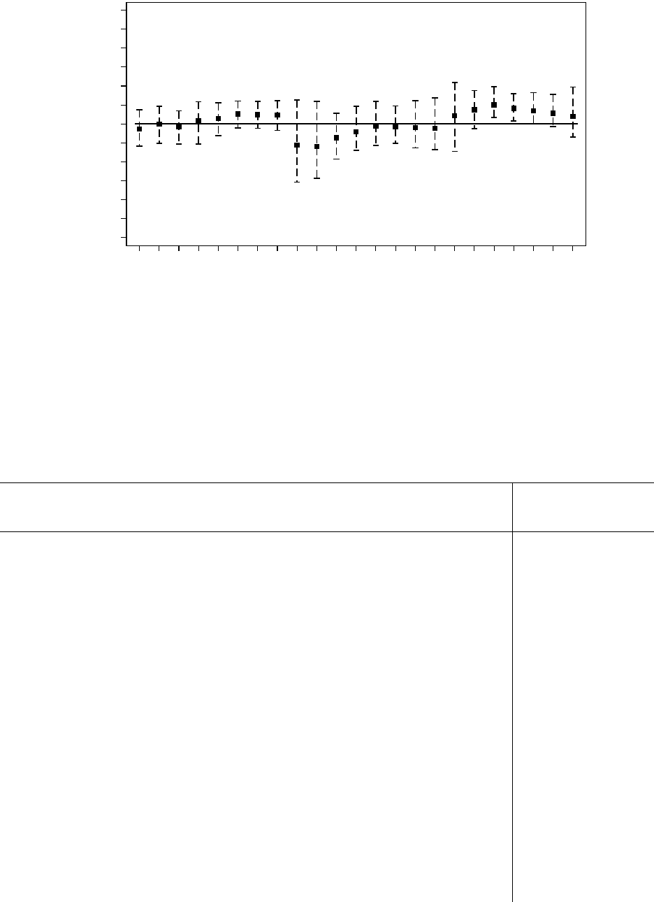
82
(b)
Figure A5.
Average treatment effect on the treated estimates with 95% confidence intervals for Models 1 through 50 of the
third analysis. Euclidian distances define the treatment and control buffers. For each ATET, the model number is followed by
the size of the treatment buffer (ft) and the size of the control buffer (ft), e.g., Model 1 has a 500’ treatment buffer and 1000’
control buffer. (a) For Models 1-27. (b) For Models 28-50. Note: confidence intervals that are out of bounds are suppressed,
e.g., for Model 1.
Table A15. Difference-in-differences and triple differences results for the third analysis, Model 62
DID
DDD
Variables
Coefficient
p-
value
Coefficient
p-value
Treatment
Blue line treatment buffer (treatment362=1)
.0218
.4658
.0398
.2532
Event
Sold after first blue line installed (event362=1)
.0185
.8296
.1012
.7396
Sensitivity
Inside 2013 XXL tsunami zone (xxl2013=1)
.1365*
.0800
Diff-in-Diff
Blue line treatment buffer (treatment362) x sold after first blue
line installed (event362)
-.0834**
.0254
-.0832
.4731
Blue line treatment buffer (treatment362) x 2013 XXL zone
(xxl2013)
-.0623
.3290
2013 XXL zone (xxl2013) x sold after first blue line installed
(event362)
-.2488
.1507
Triple Difference
Blue line treatment buffer x 2013 XXL zone x sold after first
blue line installed
-.0117
.9404
Structural
Bedrooms
.0910
.5609
.0807
.5772
Bedrooms squared
-.0188
.3282
-.0173
.3037
Bathrooms
.1256*
.0669
.1241**
.0437
Bathrooms squared
-.0055
.7158
-.0045
.7533
Indoor square footage
4.4e-04**
.0168
4.4e-04**
.0166
-.6
-.5 -.4 -.3
-.2 -.1 0
.1 .2 .3 .4 .5 .6
Coefficients
28 - 2000, 3000
29 - 2000, 3500
30 - 2000, 4000
31 - 2000, 4500
32 - 2000, 5000
33 - 2000, 5500
34 - 2000, 6000
35 - 2000, 6500
36 - 2500, 3500
37 - 2500, 4000
38 - 2500, 4500
39 - 2500, 5000
40 - 2500, 5500
41 - 2500, 6000
42 - 2500, 6500
43 - 2500, 7000
44 - 3000, 4500
45 - 3000, 5000
46 - 3000, 5500
47 - 3000, 6000
48 - 3000, 6500
49 - 3000, 7000
50 - 3000, 8000
y ( )

83
Table A15. Difference-in-differences and triple differences results for the third analysis, Model 62
DID
DDD
Variables
Coefficient
p-
value
Coefficient
p-value
Indoor square footage squared
-4.9e-08*
.0860
-5.1e-08*
.0681
Total acreage (equal to indoor area if apartment)
.0694
.7723
.1003
.6456
Total acreage squared
-.0104
.8428
-.0177
.7119
Effective age of property (2018 - remodel year)
-.0014
.6007
-.0019
.4708
Effective age of property squared
3.7e-06
.8702
7.7e-06
.7322
Heating (=1)
.2779**
.0113
.2892***
.0052
Fireplace (=1)
.0430
.3703
.0400
.4183
Garage (=1)
.0015
.9529
-.0011
.9603
Carport (=1)
-.0079
.8670
.0114
.8168
Deck (=1)
.0912
.1661
.0955
.1109
Patio (=1)
.0685
.4963
.0693
.4762
Fencing (=1)
.1049
.1486
.1041
.1461
Goal 18 eligible (=1)
-.0935
.4246
-.0892
.4680
Has shoreline armoring (=1)
.1540
.6131
.1998
.5912
Location
Special Flood Hazard Area (SFHA) (=1)
-.0085
.8749
-.0266
.6057
Elevation (ft)
5.9e-04
.2038
.0011
.1197
Elevation (ft) x Log distance to ocean shoreline x on oceanfront
(=1)
2.9e-04
.2527
2.8e-04
.2660
Slope (angular degrees of slope)
.0094
.4007
.0111
.3059
Log distance to nearest beach access point
-.0442
.1185
-.0429
.1068
Log distance to ocean shoreline
-.0799***
.0081
-.0747***
.0088
Log distance to nearest water body (lake, pond, bay)
-.0173
.4784
-.0159
.5071
Log distance to nearest river
.0167
.5020
.0201
.4495
Log distance to nearest state park or public land
.0356
.5106
.0443
.4588
Log distance to nearest national park or public land
-.0827
.1895
-.0799
.1892
Log distance to nearest highway or interstate
.0097
.7689
.0100
.7564
Log distance to nearest major road
-.0053
.6612
-.0064
.5865
Log distance to nearest railroad
-.1263
.1703
-.1240
.1558
Log distance to nearest airport
.0924
.5340
.0794
.5770
Log distance to nearest k-12 school
.0684
.4801
.0696
.4798
Log distance to nearest central business district (city)
.0134
.8239
.0085
.8788
Log distance to nearest wastewater treatment plant
.0393
.3820
.0425
.3642
Log distance to nearest fire station
.0216
.6341
.0220
.6354
Log distance to nearest law enforcement station
-.0104
.8095
-.0132
.7876
Log distance to nearest hospital
-.0150
.6977
-.0145
.67
Observations
1334
1334
Adj. R-squared
0.491
0.496
* p<0.10, ** p<0.05, *** p<0.01
