CAPITAL GAINS TAXES AND PORTFOLIO REBALANCING

issue no. 75 march 2003tiaa-crefinstitute.org

dialogue

in this issue

Introduction . . . . . . . . . . . . . . . . . . . . . . . . . . . . . . . . . . . . . . . . . . . . . . . .p 2

Model Framework . . . . . . . . . . . . . . . . . . . . . . . . . . . . . . . . . . . . . . . . . . . .p 2

Findings . . . . . . . . . . . . . . . . . . . . . . . . . . . . . . . . . . . . . . . . . . . . . . . . . .p 3

Concluding Comments . . . . . . . . . . . . . . . . . . . . . . . . . . . . . . . . . . . . . . . .p 10

Robert M. Dammon, Carnegie Mellon University

Chester S. Spatt, Carnegie Mellon University

Harold H. Zhang, University of North Carolina

The major friction that investors face in rebalancing their portfo-

lios is capital gains taxes, which are triggered by the sale of assets.

In this article, we examine the impact of an investor’s capital gains

tax liability and existing risk exposure upon the optimal portfolio

and rebalancing decisions. We capture the trade-off over the

investor’s lifetime between the tax costs and diversiﬁcation bene-

ﬁts of trading. We ﬁnd that the investor’s incentive to re-diversify

the portfolio declines with the size of the capital gain and the

investor’s age. Unlike conventional ﬁnancial advice, the reset of

the capital gains tax bases and the resulting elimination of the

capital gains tax liability at death, suggests that the optimal equity

proportion of the investor’s portfolio increases as he ages.

CAPITAL GAINS TAXES AND PORTFOLIO

REBALANCING

r esearch

> research dialogue

>>>INTRODUCTION

The major friction that investors face in rebalancing

their portfolios is capital gains taxes.

An investor who

has only capital losses can, without the payment of a

capital gains tax, rebalance his portfolio to the uncon-

strained optimal level of risk given the assumed structure

of future tax liabilities. However, for an investor with

embedded capital gains, the optimal amount of rebalanc-

ing depends upon the magnitude of these gains and the

extent of deviation of the asset holdings from the opti-

mal portfolio. The presence of these capital gains liabili-

ties inﬂuences the investor’s optimal rebalancing

decision as the investor’s optimal portfolio choice

reﬂects the trade-off between (a) realizing a certain

amount of capital gains immediately and using the liqui-

dated funds to rebalance his portfolio and (b) deferring

the realization of the remainder of the capital gains.

In this article, we examine the impact of such factors

as an investor’s capital gains tax liability and existing

risk exposure upon the optimal portfolio and rebalanc-

ing decisions in a taxable account. We capture the

trade-off over the investor’s lifetime between the tax

costs and diversiﬁcation beneﬁts of trading. We show

that an investor’s incentive to re-diversify his portfolio

declines with the size of the capital gain and his age.

Unlike conventional ﬁnancial advice, the reset of the

capital gains tax bases and the resulting elimination of

the capital gains tax liability at death suggest that the

optimal equity proportion of the investor’s portfolio

increases as he ages.

This article draws on Dammon, Spatt and Zhang

(2001a), where we formalize and solve the problem

facing an investor who derives utility (well-being) from

his intertemporal consumption levels and ﬁnal

bequest. We formulate the portfolio-rebalancing prob-

lem confronting an individual investing in taxable

accounts with an eye towards solving for the investor’s

optimal intertemporal portfolio. In this presentation

we summarize the model framework and the features

of its solution.

>>>MODEL FRAMEWORK

The Tax Environment

There are several crucial features of the tax environ-

ment that our model captures. The most important

feature is that the payment of capital gains taxes is

triggered by the sale of assets rather than the total

increase in the market value of the investor’s assets (as

in “accrual taxation” or “marking to market” the posi-

tions at the end of each tax year).

Our analysis focuses

upon the impact of taxation of capital gains at their

sale/realization on the investor’s optimal rebalancing

and asset allocation choices. It is this feature of our

setting that signiﬁcantly enhances its richness as the

investor’s optimal portfolio depends upon variables

that reﬂect the extent of the investor’s embedded gains

and his existing portfolio holdings.

Another important feature of the tax environment in

our model is the assumption that at death the investor’s

tax bases on risky assets are “reset” to their current

market values, thereby eliminating the capital gain tax

liability. This reset of the tax bases follows the actual

tax code in the United States and has an especially

important effect on the investor’s optimal portfolio

and rebalancing decisions as the investor ages and his

mortality risk increases.

Because we focus upon long-term asset allocation

issues and try to reﬂect the presence of portfolio-offset

rules that limit the degree of asymmetry between the

effective treatment of short-term and long-term real-

izations, we assume a constant tax rate for all capital

gain and loss realizations. Eliminating any distinction

between short-term and long-term realizations also

helps simplify the analysis, as we do not need to

condition the solutions upon how long the investor

has held the asset.

To summarize, the key features of our modeling of

capital gains taxation are: (a) capital gains taxes are

triggered by the sale of assets; (b) any capital gains tax

liability is forgiven at the investor’s death as the

investor’s tax basis is reset to the asset’s market value;

and (c) the capital gains tax rate does not depend upon

how long the investor has previously held the asset.

The Investor’s Problem

In order to focus upon the impact of the investor’s age

and increasing mortality, we assume that the investor

has a limited (ﬁnite) life expectancy and that the prob-

ability of survival in each period is given by an

assumed observed mortality schedule. In much of the

analysis the investor’s income is derived

only from

issue no. 75 march 2003 <

ﬁnancial assets (i.e., by assumption there is no labor

income). The investor can trade two assets—a risk-free

asset whose return is constant over time and a risky

security. The pre-tax capital gain return on the risky

asset is assumed to follow a binomial process whose

return is independent over time. The pre-tax dividend

yield is assumed constant over time.

We assume that there are no trading costs and short

sales are not permitted. Furthermore, nominal divi-

dends and interest payments are taxed at the tax rate

on ordinary income, while realized capital gains and

losses are taxed at a capital gains tax rate (which can

be lower than the ordinary income tax rate). To calcu-

late the investor’s capital gains tax we assume that

the investor’s tax basis is the weighted average

purchase price of these shares. When the risky

asset’s current price is below the investor’s tax basis,

the investor sells shares to realize the tax loss and

immediately repurchases the optimal number of

shares of the risky asset.

When the risky asset’s

current price is above the investor’s tax basis, the

new basis reflects the weighted average of the prior

basis and the current acquisition price of any new

shares acquired.

The objective of the investor’s optimization problem

is to maximize his discounted expected utility of life-

time consumption, including the utility of his

bequest at death.

Expected utility is the weighted

average utility reflecting the probability of living

through the respective dates. The treatment of

bequest is consistent with the reset provision of the

U.S. tax code under which the capital gains tax is

forgiven at death. At the beginning of each period,

the investor allocates his wealth among consump-

tion, the risk-free and risky assets, and the payment

of capital gains taxes resulting from a sale of the

risky asset. The investor is assumed to have a power

utility function so that he possesses constant relative

risk-averse preferences. (Under such a utility func-

tion, the investor will allocate the same percentage of

wealth to the risky assets regardless of his wealth

level.)

In solving the investor’s optimization problem, we

have simpliﬁed the model in order to maintain

computational tractability. For a detailed discussion of

these simpliﬁcations of the model, see Appendix.

Base-case Parameters for

Numerical Solutions

In the numerical analysis we assume that the investor

makes annual decisions starting at age 20 and lives for

up to another 80 years. The annual mortality rates are

taken from the 2000 U.S. Life Tables for the total

population.

For our base-case scenario we assume that the risk-

free (pre-tax) interest rate is 6% annually, the nominal

annual dividend yield is assumed to be a constant 2%,

and the annual inﬂation rate is 3.5%. The nominal

capital gains return on the stock follows a binomial

process with an annual mean return of 7% and stan-

dard deviation of 20%.

The tax rate on dividends and

interest is 36%, while the tax rate on capital gains is

set at 20%. The investor is assumed to have a risk

aversion parameter of 3.0 in the power utility formula-

tion with an annual discount factor of .96.

>>>FINDINGS

The “Aging Effect”

Using our base-case parameters the optimal equity

Consumption Decisions

Our setting can be used to solve for the

investor’s optimal consumption decisions. For

a given level of total wealth, the larger the

total embedded capital gain, the larger is the

investor’s implicit tax liability and the less

wealthy is the investor on an after-tax basis.

As suggested by options pricing theory, the

optimal consumption-wealth ratio and the

sensitivity of the value of the tax-timing

option decline as the size of the investor’s

capital gain increases. The optimal consump-

tion-wealth ratio also becomes less sensitive

to the size of the gain for elderly investors

due to the impending reset of the tax basis at

death. However, for the purposes of this pres-

entation we focus upon the investor’s portfo-

lio holdings rather than consumption

decisions.

> research dialogue

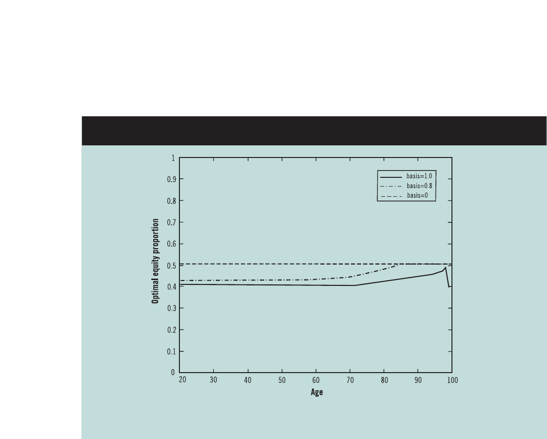
holding in the presence of capital gains taxes is illus-

trated in Figure 1, which depicts the optimal stock

proportion as a function of the investor’s age at several

different basis-price ratios, such as 1 (zero gain), 0.8

(25% gain) and 0 (entire position is gain). For our

base-case parameters the investor’s preferred equity

allocation (i.e., when the basis-price ratio equals one)

is approximately 41% if the investor is between 20 and

76 (it is higher for elderly investors). The ﬁgures are

drawn for an assumed initial stock holding of 50% of

the investor’s beginning-of-period wealth, so that the

investor is initially overexposed to equity.

An interesting feature of our solution is that the

investor’s optimal exposure to equity tends to increase

with age, particularly at late ages. This is a result of the

structure of capital gains taxation and more speciﬁ-

cally the reset of the investor’s tax basis at death. This

reset at death increases the attractiveness of retaining

highly appreciated positions, especially when the

investor’s life expectancy is relatively short. With a

short horizon, the cost of not being fully rebalanced is

small, while the tax beneﬁt of deferral is high. In this

sense the extent to which the investor scales back his

position is inﬂuenced by the interaction between his

age and the size of the capital gain.

Analogously, the investor will ﬁnd it attractive to add

relatively more equity to his portfolio as he ages (and

his life expectancy falls) because of the option to real-

ize losses, while retaining appreciated positions until

the reset at death. This observation goes beyond the

standard insight of estate planners that elderly

investors may wish to retain highly appreciated posi-

tions to defer the capital gains tax liability (e.g., until

death). In addition to addressing the investor’s behav-

ior once he possesses highly appreciated positions, our

argument also points to the beneﬁt of holding more

equity to create the option of being able to defer the

appreciated equity position (e.g., until the reset at

death) and realize positions with capital losses. This is

illustrated by the curve corresponding to the basis-

Figure 1 Optimal Stock Holding As a Function of the Investor’s Age

Note: The basis-price ratio is set at 0, 0.8, and 1, respectively.

The initial stock holding as a fraction of beginning-of-period wealth is set at 50 percent.

issue no. 75 march 2003 <

price ratio of one in Figure 1, which describes the

investor’s holdings (and purchase) of equity when the

investor is not restricted by existing capital gains.

10,11

The conventional advice on asset allocation is that an

investor should reduce his equity exposure as he

ages. In fact, some mutual fund organizations even

promote the heuristic rule that an investor’s percent-

age exposure to equity should be 100 – A, where A is

the investor’s age (in years). The underlying focus of

this perspective concerns the shortening horizon

over which the investor will utilize his funds as he

ages and the absence of nonfinancial income during

the retirement years as well as the declining value of

his human capital wealth over time during the work-

ing years.

It is not apparent that models of risk bearing without

taxes and other frictions should lead to strong age

effects about portfolio composition during the retire-

ment years. While the investor’s age and the strength

of his bequest motive will signiﬁcantly inﬂuence the

investor’s consumption decision (i.e., the shape of his

consumption path over time), the effect of age on the

allocation decision will not be pronounced as long as

the investor’s risk aversion stays constant over time.

Of course, if the investor becomes more risk averse as

he ages, then the relative demand for the risky assets

would decline with the investor’s age. Yet, many

investors with substantial wealth view themselves as

managing their funds at the margin for the beneﬁt of

their heirs, emphasizing both that risk aversion would

not increase as they age as well as the importance of

managing the capital gains tax liability efﬁciently.

Even if the investor does not have a strong bequest

motive, the investor can still ﬁnd it attractive to borrow

to help ﬁnance consumption in his latter years in

order to defer some of the capital gains liability until it

is eliminated at death (repaying the indebtedness

through his estate). More generally, our analysis high-

lights the value to the investor of borrowing in his

latter years to obtain liquidity, while deferring the real-

ization of substantial appreciated positions until the

investor’s death. While our analysis so far abstracts

from the stochastic structure of labor income, this

simpliﬁcation does not affect behavior during the

investor’s retirement years, i.e., after he has ceased

earning signiﬁcant labor income.

The Size of the Gain and Portfolio

Rebalancing

Our solutions illustrate the important role of the size of

the existing capital gain for the investor’s portfolio

rebalancing decision. If the investor is overexposed to

equity, the investor will trade off the tax cost of selling

some equity with the diversiﬁcation beneﬁt of the

reduced exposure to the risky asset. The smaller the

size of the gain, the smaller the tax costs of scaling back

the equity exposure by a given amount. Consequently,

when the size of the gain is small, the investor opti-

mizes this trade-off by scaling back equity holding to a

greater degree and getting closer to the unconstrained

optimal exposure.

Analogously, it will also be optimal

for the investor to scale back the exposure to a greater

degree when the capital gains tax rate is particularly

low. In contrast, when the size of the gain is very large

(or the tax basis is very small), the investor may just

scale back slightly or even retain the entire exposure

(the investor acts as “locked in” and does not sell his

position due to the tax cost of selling despite the risk-

sharing beneﬁts from reducing the equity exposure).

For a given size capital gain (i.e., ﬁxing the basis-price

ratio), the marginal cost to the investor of being over-

exposed to equity increases in the difference between

the size of his position and the optimal position, while

the marginal tax cost of rebalancing is constant in the

position’s size. Consequently, once the investor is

substantially overexposed to equity, the trade-off he

faces with capital gains taxes pushes him to the same

exposure, i.e., the portfolio will not depend upon his

previous holding of equity, though it depends upon

the size of the investor’s gain and age.

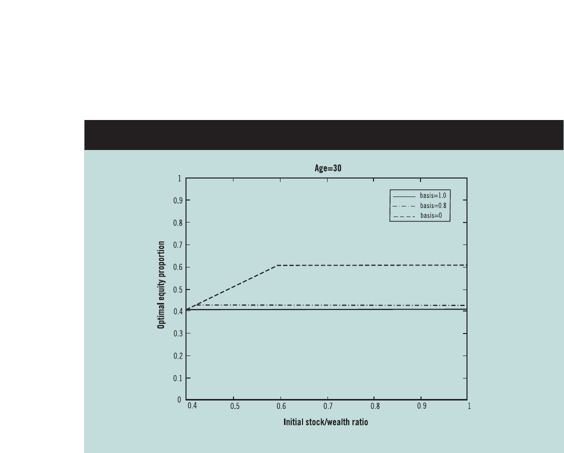
Many of these features are illustrated in Figure 2, which

depicts the optimal stock holding at age 30 for our base-

case parameters as a function of the initial proportion

of equity in the portfolio for several different values of

the basis-price ratio. The ﬁgure illustrates that the size

of the investor’s optimal equity holding increases with

the fraction of beginning-of-period wealth invested in

equity until the investor reaches his maximum expo-

sure for each basis-price ratio. The optimal equity

proportion also increases with the size of the gain (or

lower basis-price ratio) in the ﬁgure as the investor

scales back his exposure relatively less as the gain rises.

> research dialogue

Welfare Comparisons

The investor signiﬁcantly enhances the utility value of

his portfolio by efﬁciently managing his tax opportuni-

ties. We considered the welfare costs of not following

the optimal policy. Speciﬁcally, we considered the

welfare costs of the following inefﬁcient alternatives:

(a) realizing all capital gains and losses each period, or

(b) following the buy-and-hold policy of never realizing

capital gains or losses other than to ﬁnance consump-

tion.

The welfare costs reﬂect how much additional

wealth we need to provide the investor following an

alternative realization policy so that he would be as

well off as under the optimal policy. We can solve

numerically for the optimal decision rules for each of

these alternative realization policies and compare the

investor’s welfare.

The ﬁrst alternative focuses upon the advantages of

realizing losses without allowing the investor to defer

gains. The welfare costs in this case increase in the

size of the existing capital gain (since this alternative

involves selling assets with embedded gains) and

decrease in the investor’s age (due to the shortening

horizon). The welfare costs of the second alternative

(the buy-and-hold policy) decrease in the investor’s age

(again due to the shortening horizon), but now

increase in the size of the existing capital loss.

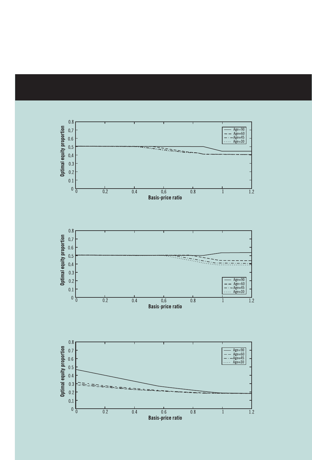
Comparative Static Analysis

We examine the impact on our policy rules of varying

the capital gains tax rate and the volatility of stock

returns. Figure 3 illustrates the optimal equity expo-

sure for our base-case parameters (upper panel), for a

tax rate of 36% on capital gains and losses (middle

panel) and for a standard deviation of equity returns

of 30% (lower panel).

These figures are constructed

assuming an initial equity proportion of 50 percent

and holding all the other parameters at their base-

case values.

An increase in the capital gains tax rate from the base-

case 20% to 36% (middle panel) reduces the size of

Figure 2 Optimal Stock Holding As a Function of the Initial Stock Holdings

Note: The basis-price ratio is set at 0, 0.8, and 1, respectively.

issue no. 75 march 2003 <

Figure 3 Optimal Stock Holding As a Function of the Basis-price Ratio:

Three Scenarios

PANEL A. BASELINE CASE

Note:

1) The investor’s age is set at 30, 45, 60, and 90, respectively.

2) The initial stock holding as a function of beginning-of-period wealth is set at 50 percent for each panel.

PANEL B. CAPITAL GAINS TAX IS RAISED FROM 20 PERCENT TO 36 PERCENT

PANEL C. STOCK RETURN VOLATILITY IS RAISED FROM 20 PERCENT TO 30 PERCENT

> research dialogue

the capital gain that the investor is willing to realize,

especially for young investors who derive the greatest

beneﬁt from rebalancing.

In addition, in the

breakeven and loss region the investor’s holding of

equity is more sensitive to the investor’s age when the

capital gains tax rate is higher.

An increase in the volatility of the stock from the base-

case 20% to 30% (lower panel) has a dramatic impact

on the investor’s equity holdings. Not surprisingly, the

increase in riskiness of equity reduces the optimal

holdings for all investors depicted in the ﬁgure despite

the increase in the value of the tax-timing option.

However, in some circumstances elderly investors

with large gains can retain their equity exposure to

avoid the capital gains tax at death. The beneﬁts of

rebalancing are greater in a more volatile environment

so that young and middle-aged investors will cut their

exposure to equity, even when their embedded gains

are large. The ﬁndings associated with an increase in

volatility are similar to those that would arise from

increasing the investor’s risk aversion.

Mandatory Capital Gains Taxation

at Death

An interesting benchmark for comparison of our asset

allocation results is the treatment of capital gains at

death in Canada. Under the Canadian law the ability to

defer the capital gains tax ends at death. Unrealized

capital gains are automatically taxed in Canada at

death rather than beneﬁting from either (a) a step-up

in the investor’s tax basis to eliminate the capital gains

tax liability, or (b) allowing the investor to defer the tax

payment by delaying the sale of the equity and retain-

ing the prior tax basis.

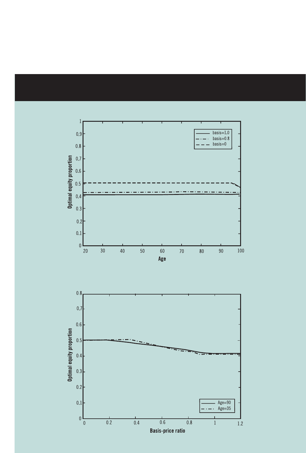
Using our base-case parameters, an initial equity

proportion of 50 percent of the investor’s beginning-

of-period wealth, and full taxation of capital gains at

death, we illustrate in Figure 4 the optimal exposure

to equity under the Canadian law. The upper panel of

Figure 4 depicts the optimal stock proportion as a

function of the investor’s age at several different

basis-price ratios, such as 1 (zero gain), 0.8 (25%

gain) and 0 (entire position is gain). Notice that the

optimal equity exposure is now relatively insensitive

to the investor’s age because there is no opportunity

to escape the capital gains tax at death and so the tax

benefit to deferral of capital gains largely reflects the

time value of money and is nearly constant over

time. This figure strongly suggests that the aging

effects in portfolio holdings in our basic analysis are

driven by the reset provision at death rather than

other features of our setting such as the specific

details of the bequest motive.

We illustrate in the lower panel of Figure 4 the impact

of the size of the gain upon the investor’s rebalancing

decision by plotting the optimal exposure to equity as

a function of the basis-price ratio for investors at ages

35 and 90 in our modiﬁed setting without the reset at

death. This highlights the nature of the rebalancing

decision across tax bases and the tradeoff between the

tax costs and risk-sharing beneﬁts, even absent the

potential for eventual reset of the tax basis at death.

Labor Income

While an important component of an investor’s wealth

and risk is determined by human capital, our earlier

analysis did not incorporate labor (non-ﬁnancial)

income. Though ideally one would like to model labor

income with its own stochastic speciﬁcation, we intro-

duce the investor’s labor income as proportional to his

wealth so as to avoid the need to increase the dimen-

sionality of our model. This allows us to capture

several fundamental aspects of the impact of non-

ﬁnancial income on asset allocation over the life cycle

in the presence of taxes. For example, investors

younger than age 65 (when we assume that the labor

income terminates) substantially increase their opti-

mal holding of equity relative to the case without labor

income. This is in response to the increase in the

investor’s effective wealth and the modest risk of non-

ﬁnancial income. Consequently, human capital and

the reset provision have the opposite effects on the

optimal equity exposure as a function of the investor’s

age. Of course, the human capital effect is typically

present only when the impact of the reset beneﬁt

provision is weakest (i.e., at young ages).

An important aspect of non-financial income is that

by enhancing the investor’s income stream only in

his working years there is a greater flow of new

savings. This greater flow of new savings helps limit

the extent to which the investor becomes locked in

and allows the investor to rebalance his portfolio

without payment of capital gains taxes by altering the

portfolio allocation of new investments. In practice,

issue no. 75 march 2003 <

Figure 4 Optimal Stock Holding Under Mandatory Capital Gains Taxation

At Death

Note:The initial stock holding as a fraction of beginning-of-period wealth is set at 50 percent for both panels.

PANEL A. OPTIMAL STOCK HOLDING AS A FUNCTION OF THE INVESTOR’S AGE

PANEL B. OPTIMAL STOCK HOLDING AS A FUNCTION OF THE BASIS-PRICE RATIO

AT AGE 35 AND 90, RESPECTIVELY

> research dialogue

incremental savings over time creates the ability to

adjust the structure of one’s portfolio.

>>>CONCLUDING COMMENTS

Our framework provides a tractable way to capture the

trade-off between the payment of capital gains taxes

and portfolio rebalancing. We demonstrate how an

investor’s optimal portfolio holdings depend upon the

investor’s age, existing capital gain and portfolio hold-

ings. For an investor with embedded capital gains, the

incentive to rebalance his portfolio by selling stock is

inversely related to his age and the size of the gain.

Elderly investors have a strong incentive to defer the

realization of existing capital gains and to increase

their ownership of equity as they age due to the

forgiveness of capital gains taxes at death under the

current U.S. tax code.

In addition to the substantive qualitative insights that

emerge from our analysis, our study also makes a

methodological contribution. Our work provides a

tractable way to incorporate a realistic treatment of

capital gains taxes in the analysis of asset allocation.

Most directly, we have extended the analysis to incor-

porate two risky securities in Dammon, Spatt and

Zhang (2001b).

Building upon our framework we also have introduced

in Dammon, Spatt and Zhang (2002a) the opportunity

for tax-deferred investing into an integrated asset allo-

cation setting.

Our work emphasizes the value of

optimal asset

location (which assets to hold in which

account) in addition to optimal asset allocation. The

implications of our framework for estate planning

issues, including the titling of securities by a married

couple and the location of exposures between trusts

and personal assets, are explored in Dammon, Spatt

and Zhang (2002b).

>>>ACKNOWLEDGEMENTS

This paper builds off Dammon, Spatt and Zhang

(2001a), which was partially supported by the TIAA-

CREF Institute and received the Michael Brennan

(Runner-up) Prize of the Review of Financial Studies.

The views expressed in this article are those of the

authors’ alone and are not necessarily those of TIAA-

CREF or any member of its staff.

issue no. 75 march 2003 <

>>>APPENDIX

The inherent difﬁculty in solving the underlying prob-

lem is that the investor’s decisions depend upon the

investor’s existing portfolio holdings, speciﬁcally his

holdings of the risky asset and its respective tax basis.

In this sense the investor’s underlying expected utility

maximization problem is fundamentally dynamic. We

can recast this model recursively as a dynamic program-

ming problem. While numerical methods can be used

to solve such dynamic programming problems, it is

crucial to the tractability of these problems that there

are only a small number of underlying “state variables,”

upon which the optimal decision rules are functions.

We identify several simpliﬁcations to help limit the

number of state variables, so that the problem is

tractable numerically. An important additional advan-

tage of these simpliﬁcations is that they highlight the

variables that are central to understanding the solu-

tions, thereby focusing the reader upon the funda-

mental aspects of the problem.

In the underlying problem the state variables include

the tax basis (and distinct purchase price) for the risky

asset and the corresponding size of that position as

well as the investor’s wealth. To simplify the problem

and highlight the key underlying intuitions, we restrict

attention to a problem with a single risky asset and a

risk-free asset.

The average basis can be updated using the investor’s

prior average basis so that assuming an average basis

rule greatly limits the dimensionality of the underly-

ing state space and helps makes it tractable to obtain

numerical solutions. Indeed, mutual funds report to

investors the basis of their holdings using the aver-

age basis rule, which is a heuristic used by many

investors. In Canada the actual tax liability is deter-

mined by an average basis rule. While this averaging

rule is not optimal for the United States tax code

(e.g., with constant tax rates over time it is optimal

for the investor to realize the highest basis positions

first), most of the qualitative features that emerge

from our solutions reflect robust features of the solu-

tion to the investor’s optimization problem. In addi-

tion, DeMiguel and Uppal (2002) present numerical

results suggesting that the value of the investor’s

optimal solution is not substantially larger under the

optimal policy than when using the averaging rule.

Finally, specializing the investor’s preferences to

constant relative risk aversion (power utility) ensures

that the resulting demands for the risky (and risk-free)

asset as well as consumption are proportional to

wealth. Consequently, we can treat the beginning-of-

period wealth as the numeraire to normalize wealth

out of the consumption and portfolio choice problems

and solve for the fraction of the investor’s wealth that

is allocated to current consumption, the risky asset

and the risk-free asset. Imposing the overall budget

constraint, this leads to two independent choice vari-

ables. The optimal asset allocation (the proportion of

assets allocated to the risky security) and consumption

decisions are functions of the investor’s current asset

allocation, average tax basis and age. As a result, the

problem can be expressed with two continuous state

variables as well as age.

REFERENCES

Chari, V.V., M. Golosov, and A. Tsyvinski, 2002,

“Business Start-ups, the Lock-in Effect, and Capital

Gains Taxation,” unpublished working paper,

University of Minnesota and Federal Reserve Bank of

Minneapolis.

Constantinides, G., 1983, “Capital Market Equilibrium

with Personal Tax,” Econometrica, 51, 611-636.

Constantinides, G., 1984, “Optimal Stock Trading with

Personal Taxes: Implications for Prices and the

Abnormal January Returns, Journal of Financial

Economics, 13, 65-89.

Dammon, R., and C. Spatt, 1996, “The Optimal

Trading and Pricing of Securities with Asymmetric

Capital Gains Taxes and Transaction Costs,” Review of

Financial Studies, 9, 341-372.

Dammon, R., C. Spatt, and H. Zhang, 2001a,

“Optimal Consumption and Investment with Capital

Gains Taxes,” Review of Financial Studies, 14, 583-616.

Dammon, R., C. Spatt, and H. Zhang, 2001b,

“Diversiﬁcation and Capital Gains Taxes with Multiple

Risky Assets,” unpublished working paper, Carnegie

Mellon University and the University of North

Carolina.

Dammon, R., C. Spatt, and H. Zhang, 2002a,

“Optimal Asset Location and Allocation with Taxable

and Tax-Deferred Investing,” unpublished working

paper, Carnegie Mellon University and the University

of North Carolina.

Dammon, R., C. Spatt, and H. Zhang, 2002b, “Taxes,

Estate Planning and Financial Theory: New Insights

and Perspectives,” unpublished working paper,

Carnegie Mellon University and the University of

North Carolina.

DeMiguel, A., and R. Uppal, 2002, “Portfolio

Investment with the Exact Tax Basis via Nonlinear

Programming,” unpublished working paper, London

Business School.

Dybvig, P., and H. K. Koo, 1996, “Investment with

Taxes,” unpublished working paper, Washington

University in St. Louis.

> research dialogue

Fama, E., and K. French, 2002, “The Equity Premium,”

Journal of Finance, 57, 637-659.

Gallmeyer, M., R. Kaniel, and S. Tompaidis, 2001,

“Two Stock Portfolio Choice with Capital Gains Taxes

and Short Sales,” unpublished working paper,

University of Texas at Austin.

Garlappi, L., V. Naik, and J. Slive, 2001, “Portfolio

Selection with Multiple Assets and Capital Gains

Taxes,” unpublished working paper, University of

British Columbia.

Poterba, J., 2001, “Estate and Gift Taxes and Incentives

for Inter Vivos Giving in the US,” Journal of Public

Economics, 79, 237-264.

issue no. 75 march 2003 <

ENDNOTES

The magnitude of direct trading costs has declined

substantially in recent years as reflected by the

huge drop in commissions and the dramatic

reduction in tick size brought about by decimaliza-

tion. In most situations facing taxable investors

the major component of trading costs is capital

gains taxes.

This article examines investing in the investor’s

taxable account, but does not incorporate tax-

deferred investing. Tax-deferred investing in a

setting with capital gains taxation in the taxable

account is examined in Dammon, Spatt and Zhang

(2002a) and brieﬂy referenced in the concluding

comments of this article.

The effect of taxing capital gains upon asset realiza-

tions was ﬁrst explored in Constantinides (1983,

1984). Both these papers focus upon the value of

harvesting capital losses. Constantinides (1984) also

addresses the optimality of harvesting gains at pref-

erential (long-term) capital gains tax rates under

some circumstances.

Our assumption of symmetric treatment of short-

term and long-term realizations is particularly natu-

ral in light of the interpretation of a period being

one year when we parameterize and implement our

model. An interesting dynamic analysis of optimal

gain and loss harvesting in the presence of asym-

metric treatment of short-term and long-term real-

izations is given in Dammon and Spatt (1996),

though they do not address the intertemporal port-

folio problem of a risk-averse investor. The value of

realizing long-term gains to create the option of

realizing future short-term losses was ﬁrst explored

in Constantinides (1984).

Throughout our analysis we assume that there are

no transaction costs and no wash sale restrictions

on realizing losses (in practice, investors must defer

the realization of the tax loss if they repurchase the

same position within 30 days of realizing the loss).

For example, wash sale rules are not very restrictive

in practice given the existence of close substitute

securities that can be repurchased immediately after

a sale of the security in question without triggering

wash-sale treatment. Consequently, it is optimal in

our model for the investor to sell his entire position

when he has a loss and then repurchase the optimal

risky exposure.

The bequest function at death is based upon the

investor providing his beneﬁciary with a uniform

real consumption stream over H periods.

While we are using an aggregate mortality curve for

illustration, a particular investor should use his

own life expectancy based upon gender and health

information.

The resulting risk premium is (1.07)(1.02)-1.06 =

.0314 = 3.14%, which is well below the historical

average. This reﬂects our desire that the investor

optimally owns bonds as well as equity for reason-

able levels of risk aversion. Our choice of risk

premium is consistent with the perspectives of

many ﬁnancial economists about anticipated future

risk premium, as illustrated by the analysis of Fama

and French (2002).

These base-case parameters are the same as in the

base-case in Dammon, Spatt and Zhang (2001a),

except that we have replaced the mortality schedule,

the capital gains tax rate here is 20% rather than

36%, and the standard deviation is 20% rather than

20.7%.

The curve corresponding to the basis-price ratio of

one does not continue to rise at age 99 in Figure 1

because we do not allow the investor to realize

losses at the time of death.

Our analysis understates the value of holding

equity in several respects. Because we focus upon

a single security and treat its basis as the average

acquisition cost, the investor does not have the

ability to treat the tax basis of new shares as the

acquisition price. Instead, the option value of these

positions is limited because they are being blended

with the investor’s previously acquired appreciated

positions. If the investor’s prior appreciation is

substantial, then our solutions do not illustrate

fully the benefit that arises from newly acquired

positions. However, if the basis-price ratio equals

one then the increasing proportion of equity in the

investor’s portfolio as he gets older illustrates to a

> research dialogue

At age 90 the investor actually adds equity when the

capital gains tax rate is 36% due to the extent of the

beneﬁt of the reset provision at death for this tax rate.

The introduction of each additional risky asset

requires two additional continuous state variables

(one for the asset’s proportion and another for its

basis). Related analyses of the asset allocation prob-

lem with two risky assets that utilize the framework

developed in Dammon, Spatt and Zhang (2001a)

are Gallmeyer, Kaniel and Tompaidis (2001) and

Garlappi, Naik and Slive (2001). As discussed in the

Appendix, the curse of dimensionality impedes

greatly the introduction of additional state variables

(and assets).

Because the reset of the investor’s tax basis at death

does not arise within the tax-deferred account, the

aging effects we emphasize here do not arise within

that account.

Since we want our numerical solution to be rela-

tively smooth, we need to solve the underlying prob-

lem on a relatively dense grid. The resulting

computational demands then expand exponentially

with the number of state variables and our formula-

tion suffers from the curse of dimensionality.

Even using a risk-free asset and a single risky asset

whose return follows a binomial process, Dybvig

and Koo (1996) were able to solve the full-blown

optimization problem for a risk-averse investor

using the entire distribution of bases only for hori-

zons up to four periods.

greater degree the underlying tax benefit of

increasing his exposure to equity.

A simple example of this point is illustrated by the

case without taxes in which the investor has an

additive separable log utility function over his

consumption each period as well as the annuitized

amount of his real bequest. In each period the

investor’s allocates his portfolio to maximize the log

of his one-period ahead wealth.

Poterba (2001) documents that elderly investors

with low embedded capital gains have a greater

propensity to gift assets to their heirs during their

lifetimes as compared to investors with substantial

capital gains and equivalent wealth, reﬂecting the

interest of investors with large capital gains in

utilizing to a greater degree the reset of the tax

bases at death.

Our model also can produce situations in which the

investor’s optimal future proportion of equity is

increasing in the size of his earlier capital gain

when the investor initially owns less equity than his

optimal level. When the investor is underexposed in

his equity holding a larger gain can reduce the

amount of additional equity purchased by the

investor because the basis of his newly acquired

shares will reﬂect the averaging with existing shares

with substantial appreciation. This situation is illus-

trated by numerical solutions in Dammon, Spatt

and Zhang (2001a). We do not emphasize this

conclusion in the presentation here because it

reﬂects an artifact of the average basis rule that we

use to facilitate numerical solutions rather than a

general feature of the optimal capital gains problem

with risk-averse investors.

An alternative context in which the welfare conse-

quences of the capital gains tax is explored is in

Chari, Golosov, and Tsyvinski (2002), who suggest

that there are substantial distortionary consequences

of capital gains taxation for entrepreneurial activity.

Our base-case standard deviation is representative

of the annual volatility of the market index, while

increasing the standard deviation to 30% makes the

standard deviation representative of that of individ-

ual stocks.

730 Third Avenue

New York, NY 10017-3206

Tel 800.842.2733 ext 6363

tiaa-creﬁnstitute.org