
1
Hospital Network Competition and Adverse Selection:
Evidence from the Massachusetts Health Insurance Exchange
Mark Shepard
*
Harvard Kennedy School and NBER
February 29, 2016
Abstract
I study the role of adverse selection when health insurers compete on an increasingly
important benefit: coverage of the most prestigious (and expensive) “star” hospitals.
Using data from Massachusetts’ pioneer insurance exchange, I show evidence of
substantial adverse selection through a channel theoretically distinct from standard
selection on medical risk. Plans that cover star hospitals attract consumers with high costs
because when sick, they tend to use the expensive star providers. This selection persists
even with risk adjustment, which does not offset higher costs driven by hospital choices
rather than medical risk. I show evidence of adverse selection through this mechanism
using consumer choices across plans that differ in star hospital coverage and using
switching choices after a plan drops the star hospitals from network. I then estimate a
structural model of insurer competition to study the welfare and policy implications of
selection. I find that adverse selection creates a strong incentive not to cover the star
hospitals. Simple modifications to risk adjustment can preserve coverage, but I find that
they do little to improve net welfare because of offsetting costs of greater use of the star
hospitals. These results illustrate the challenge of addressing adverse selection in settings
where it is linked to moral hazard.
*
Post-Doctoral Fellow in Aging and Health Care at NBER (2015-16) and Assistant Professor of Public Policy at
Harvard Kennedy School (2016+). Email: Mark_She[email protected]ard.edu. I thank my Ph.D. advisors David
Cutler, Jeffrey Liebman, and Ariel Pakes for extensive comments and support in writing this paper. I thank the
Massachusetts Health Connector (and particularly Michael Norton, Sam Osoro, Nicole Waickman, and Marissa
Woltmann) for assistance in providing and interpreting the data. I also thank Katherine Baicker, Amitabh Chandra,
Jeffrey Clemens, Keith Ericson, Amy Finkelstein, Jon Gruber, Kate Ho, Sonia Jaffe, Tim Layton, Robin Lee, Greg
Lewis, Tom McGuire, Joe Newhouse, Daria Pelech, Amanda Starc, Karen Stockley, Rich Sweeney, Jacob Wallace,
Tom Wollmann, Ali Yurukoglu, and participants in seminars at Boston College, the Boston Fed, CBO, Columbia,
Chicago Booth, Duke Fuqua, Harvard, the NBER Summer Institute, Northwestern, U Penn, Princeton, Stanford
GSB, UCLA, UCSD, and Washington University for helpful discussions and comments. I gratefully acknowledge
data funding from Harvard’s Lab for Economic Applications and Policy, and Ph.D. funding support from National
Institute on Aging Grant No. T32-AG000186 (via the National Bureau of Economic Research), the Rumsfeld
Foundation, and the National Science Foundation Graduate Research Fellowship.

2
Introduction
Public programs increasingly use regulated markets to provide health insurance to enrollees. These types
of markets now cover more than 75 million people and cost over $300 billion in U.S. programs including
the Affordable Care Act (ACA), Medicare Advantage, and Medicaid managed care. Markets can improve
welfare by giving consumers choice and encouraging insurer competition. But a perennial concern in
insurance markets is adverse selection. When high-cost types tend to prefer generous plans, insurers may
have inefficient incentives to cut benefits to avoid attracting these customers. Selection is a particular
concern in regulated markets because – to promote goals of equity and long-term insurance (Handel,
Hendel, and Whinston 2013) – regulators typically restrict insurers from pricing on health status or most
other observable variables. Instead, regulators use a tool called “risk adjustment” that transfers payments
among insurers to compensate plans that attract observably sicker groups. They also regulate plan
attributes, including cost sharing and covered services, to prevent a race to the bottom in these benefits.
A natural question is whether adverse selection still matters in these heavily regulated and risk-
adjusted markets. In this paper, I address this question for an increasingly important benefit: insurers’
networks of covered hospitals and other medical providers. Despite a large literature on selection, there is
little direct evidence on whether plans with better networks face adverse selection.
1
This question is
particularly important in regulated markets like the ACA exchanges, where networks are one of the few
benefits on which insurers can flexibly compete.
2
The first years of the ACA have seen a proliferation of
“narrow network” plans, which comprise almost half of exchange plans (McKinsey 2015).
3
These plans have generated controversy, including calls for broader network requirements, partly
because they tend to exclude the most prestigious academic hospitals.
4
These “star” hospitals are known
as centers of advanced medical treatment and research but, partly as a result, are quite expensive (Ho
2009). By excluding them, insurers limit access to top providers but also reduce costs by steering patients
to cheaper settings. However, insurers’ incentives to balance this cost-quality tradeoff may also be
influenced by adverse selection. Whether selection is involved is an important question for assessing the
trend towards narrow networks and for the policy debate.
1
The literature has focused on selection between plans with higher vs. lower cost-sharing (e.g., deductibles) and
between HMOs and traditional fee-for-service (FFS) plans (see Glied 2000 for a review). HMOs often have
narrower networks than FFS plans but also differ in a variety of other managed care restrictions.
2
The ACA heavily restricts covered services and cost-sharing rules. All plans must cover a broad set of “essential
health benefits.” Cost sharing generosity must fall within four tiers (bronze/silver/gold/platinum), and insurer
flexibility is further limited by “cost-sharing subsidies” that limit cost sharing for enrollees below 250% of poverty.
3
McKinsey defined narrow network plans as those excluding at least 30% of area hospitals. They documented a
sharp increase in the share of narrow network plans relative to pre-ACA insurance markets.
4
An article in U.S. News & World Report found that of that publication’s top 18 ranked hospitals nationwide, 14
were covered by a minority of insurers on their state’s exchange in 2014 (Richards 2013). This stands in contrast to
employer-sponsored insurance, where star hospitals are often viewed as “must-cover” hospitals.

3
Using data from Massachusetts’ pioneer insurance exchange, I show evidence of substantial
adverse selection against plans that cover the state’s top-ranked star hospitals. This selection occurs partly
through a channel that is theoretically distinct from the usual selection mechanism and therefore poses a
challenge for standard policy tools. Typically, economists equate adverse selection with high-risk (sicker)
people selecting certain plans. But in addition to medical risk, some consumers may be more costly
because for a given illness, they tend to choose expensive providers. This second dimension is likely to be
important, since provider prices vary widely within areas (IOM 2013), and insurers typically cover the
bulk of these price differences rather than passing them onto patients.
5
As a result, consumers who use
star hospitals when sick are more costly than consumers who use less expensive alternatives. I find that in
addition to classic selection on medical risk, plans that cover the star hospital face adverse selection on
this alternate (provider choice) dimension of costs.
In some ways, the implications of this alternate selection channel are standard: inefficient sorting
for consumers and incentives for insurers to avoid offering generous plans. For instance, some consumers
might value access to a star hospital should they get seriously ill, but would be otherwise unlikely to use
it. But to buy a plan covering it, they have to pool with people who regularly use star providers for all
their health care needs. Plans covering star hospitals differentially attract these high users, forcing them to
raise prices and further crowd out infrequent users. Depending on the market structure and type
distribution, this process can either stabilize or lead to unravelling of star hospital coverage.
But selection on likelihood to use star providers is non-standard for at least three reasons. First,
even excellent risk adjustment is unlikely to offset it, since provider choices are affected by many non-
risk factors. For instance, patient preferences – e.g., existing relationships with providers, patient location,
and value for quality vs. convenience – can be thought of as omitted variables in standard risk adjustment.
Thus, adverse selection is likely to remain a concern even in markets with risk adjustment.
Second, the high costs of people who prefer star hospitals are not fixed but occur only when given
the option to use these expensive hospitals at the insurer’s expense. Stated differently, these individuals
exhibit large cost increases – or moral hazard effects – when an insurer covers the star provider. What I
find is that the people most likely to use star hospitals when covered (i.e. highest moral hazard) tend to
select into plans that cover them. Thus, my findings are an example of “selection on moral hazard,” an
idea introduced by Einav et al. (2013).
6
My results suggest a natural mechanism for selection on moral
hazard whenever insurers compete on coverage of specific benefits (e.g., a star hospital or an expensive
5
The Massachusetts exchange requires plans to fully cover price differences by mandating equal copays for all in-
network hospitals. However, insurers typically cover most price differences even in less regulated settings (see e.g.,
Gowrisankaran et al. (2015) who find that patients pay just 2-3% of price differences as coinsurance in their
employer insurance setting).
6
Similar to this paper, Einav et al. (2015) show that when moral hazard effects vary, risk adjustment cannot fully
offset cost heterogeneity. They describe this as the missing “economic content of risk scores.”

4
drug or treatment option). People with the strongest preference for the expensive benefit both use it more
when sick and (anticipating this) purchase a plan that covers it.
7
Offsetting this selection channel would
require charging fees related to how much enrollees use the expensive benefit – either via higher “tiered”
copays at point of use, or via individually varying plan premiums (Bundorf et al. 2012).
A final difference from the standard analysis is that the selection is linked to a service (care at star
hospitals) whose prices are not set competitively. Instead, these prices are partly driven by star hospitals’
market power in negotiations with insurers. Because adverse selection reduces insurer incentives to cover
star hospitals, it may have the side effect of disciplining star hospital prices in exchanges (relative to
employer insurance settings where workers typically have fewer plan choices). Although I do not fully
analyze hospital-insurer bargaining in this paper, this conceptual point has important implications for
standard policy responses to selection. For instance, a mandate to cover the hospitals would be
problematic because it would give star hospitals extreme power to raise prices.
To study these issues empirically, I use data from a market that was a key model for the ACA:
Massachusetts’ subsidized insurance exchange.
8
This exchange provides a nice setting for studying
networks and selection. Exchange regulations required standardized cost sharing and covered services,
which lets me compare plans that are nearly identical except for their provider network. Further, the state
has a clear set of star academic hospitals: Mass. General and Brigham & Women’s hospitals, the flagships
of the Partners Healthcare System. U.S. News & World Report consistently ranks these as the top two
hospitals in the state and among the top 10 hospitals in the nation. Consistent with past reports (e.g.,
Coakley 2013), I find that the star hospitals are extremely expensive – with severity-adjusted prices per
admission almost twice the average of other hospitals and over $5,000 (or 33%) more than the average of
other academic medical centers. Finally, the exchange has administrative enrollment and claims data for
all consumers and plans over its entire history. These detailed data let me link plan choices, hospital
choices, and costs to study the relationships driving adverse selection.
I start by testing for adverse selection against plans covering Partners using reduced form
methods. I show that these plans attract a group who appear to strongly prefer Partners: people who have
used Partners hospitals in the past for outpatient care, which includes doctor visits and other outpatient
treatments. Compared to the average other enrollee, these past Partners patients are (1) 28% higher cost
even after risk adjustment, (2) 80% more likely to select a plan that covers Partners, and (3) almost five
times as likely to use the star hospitals for subsequent hospitalizations. These facts suggest that Partners
7
This mechanism is embedded in the standard “option demand” model of provider networks and plan choices
(Capps, Dranove, and Satterthwaite 2003; Town and Vistnes 2001) but to my knowledge has not been previously
highlighted.
8
This setting is distinct from Massachusetts’ unsubsidized exchange, which Ericson and Starc (2013, 2014, 2015)
have studied. The limited past work on the subsidized exchange by Chandra et al. (2011; 2014) has studied the
effects of the individual mandate’s introduction and of cost-sharing changes in 2008.

5
patients are loyal to their preferred hospitals and select plans partly based on their desire to continue using
these providers. I find that this loyalty to previously used hospitals is true more broadly across all
hospitals in my data, suggesting that it is a general phenomenon likely to drive plan choices in health
insurance markets.
9
This loyalty in turn matters for costs when a patient is loyal to an expensive provider.
I next study how this selection played out in a case in 2012 when a large plan dropped Partners
(both hospitals and affiliated physicians) as well as several other hospitals from its network. This type of
network change provides a natural source of evidence that has rarely been available in past research.
Consistent with the selection story, I find that high-cost Partners patients were far more likely to switch
plans in response to this change. Nearly 40% of them switched plans in 2012, compared to a switching
rate of less than 5% for enrollees who had not been patients at a dropped hospital. These switchers had
high-cost even among past Partners patients, with risk-adjusted 2011 costs 80% higher than the average
person who did not switch out of the plan. These findings suggest that many consumers are able to
overcome well-known inertia in plan switching (see Handel 2013) in order to maintain access to their
preferred doctors and hospitals. It further suggests that excluding a star hospital from network may be a
powerful tool for insurers to reduce demand among their highest-cost consumers.
I also use the 2012 network change to show evidence of moral hazard from Partners coverage that
is differentially large for past Partners patients. Using panel regressions with individual fixed effects, I
find sharp cost reductions at the start of 2012 for Partners patients who stayed in the plan that dropped
Partners. Cost reductions for all other stayers were much more modest. Thus, consistent with my model’s
prediction of “selection on moral hazard,” the same group most likely to switch plans also experienced
the largest cost reductions when they stayed with the plan that dropped the star hospitals.
The reduced form results suggest that adverse selection based on star hospital coverage is an
important phenomenon. To further investigate the welfare and policy implications of this selection, I
estimate a structural model of consumer preferences, insurer costs, and insurer competition. The model –
which follows a structure used in past work (e.g., Capps et al. 2003; Ho 2009) – consists of three pieces:
(1) a hospital demand system capturing hospital choices under different plan networks, (2) an insurance
demand system capturing plan choice patterns, and (3) a cost model estimated from the insurance claims
data. Relative to past work, the main innovation is to allow for detailed preference heterogeneity and use
the individual-level data to capture the correlations among hospital choices, plan preferences, and costs –
which are critical for adverse selection. In addition, I pay special attention to the identification of the
9
It is less clear how much of this loyalty is driven by state dependence (a preference for hospitals used in the past)
versus more durable preference heterogeneity. Both are valid channels for the short-run adverse selection results I
find. But state dependence implies lower long-run welfare impacts of unraveling of Partners coverage, since patients
need only incur a one-time cost of switching providers. Disentangling the roles of state dependence versus
heterogeneity in loyalty to providers is an important question for future research.
6
premium and network coefficients in plan demand, using only within-plan variation to identify them. For
premiums, I use variation driven by Massachusetts’ income-varying subsidy rules. For networks, I use
variation across consumers in how they value a given hospital network.
My demand estimates imply that individuals value both lower prices and better hospital networks
(including star hospital coverage), though with significant heterogeneity in this tradeoff. Consistent with
the reduced form evidence, I find that past patients of a hospital are particularly likely to use it again and
to select plans that cover it. These effects are particularly strong for past patients of Partners hospitals.
Thus, the demand estimates are consistent with significant selection based on coverage of the prestigious
Partners hospitals. Applying the model to the 2012 network change discussed above, I find that selection
explains between a third and half of the risk-adjusted cost reductions for the plan that dropped Partners.
I next use the model to study the competitive, welfare, and policy implications of network-based
selection. I simulate equilibrium in a game where insurers first choose whether or not to cover the star
Partners hospitals (holding fixed other hospital coverage) and then compete on prices. I model exchange
policies similar to those in the ACA, which differ in several ways from those used in Massachusetts. The
key limitation of these simulations is that they hold hospital prices fixed at their observed values, not
modeling hospital-insurer price bargaining. At the star hospitals’ observed high prices, I find a unique
equilibrium in which all plans drop them from network. As in the reduced form results, a plan deviating
to cover Partners loses money both through higher costs for its existing enrollees (moral hazard) and by
attracting high-cost enrollees who particularly like Partners (adverse selection). I use the model to
decompose the adverse selection into traditional selection on levels of cost and selection on moral hazard
from covering Partners. Of the substantially higher risk-adjusted costs for the group that most values
Partners, about 60% is driven by higher cost levels (i.e., even in a plan that does not cover Partners), and
40% is driven by larger cost increases when Partners is covered. Thus, both traditional selection and the
theoretically distinct form of selection are quantitatively important in this market.
Finally, I use my model to analyze policy changes to address adverse selection. I find that
modified risk adjustment and differential subsidies for higher price plans can reverse the unraveling of
star hospital coverage. These policies give plans a greater incentive to cover these hospitals even though
doing so requires raising prices and attracting high-cost enrollees. However, I highlight two tradeoffs.
First, covering the star hospitals increase costs due to moral hazard. My model’s estimates imply that past
Partners patients have greater value of access than costs, but other enrollees on average do not. Because
the latter group is much larger, I find a net decrease in social surplus when the government changes policy
to encourage Partners coverage.
A second tradeoff of these policy changes is that they encourage both insurers and Partners
hospitals to raise prices. My current model does not capture the higher Partners prices (which are held
7
fixed by assumption). But I find important increases in insurance prices and markups, leading to a
government-funded increase in insurer profits. This analysis aligns with recent work finding that adverse
selection leads plans to reduce markups in imperfectly competitive markets (Mahoney and Weyl 2014;
Starc 2014). Adverse selection gives insurers an incentive to keep prices low to attract low-cost
consumers. Policies that offset this effect encourage plans to raise price markups. In exchanges, higher
plan prices mean higher government subsidies, which are set based on these prices.
These results suggest that standard policies used to address adverse selection (e.g., risk
adjustment and subsidies) are less effective at improving welfare with selection based on star hospital use.
These policies compensate insurers for attracting high-cost enrollees but do not address the fundamental
issue of efficiently sorting patients across hospitals. Policies that address this sorting challenge directly –
e.g., higher “tiered” copays for high-price hospitals or payment incentives for doctors to steer patients to
lower-cost hospitals – may be more effective and are a fruitful subject for future research.
The remainder of this paper is organized as follows. Section 1 outlines a simple model that
captures the main intuition for network-based selection. Section 2 presents background on the
Massachusetts exchange and hospital market and introduces the data. Section 3 shows reduced form
results, and Sections 4-5 present the structural model and estimates. Section 6 analyzes the model’s
implications for adverse selection, and Section 7 presents the equilibrium and counterfactual policy
simulations. The final section concludes.
1 Basic Theory
In this section, I present a simple model to illustrate how coverage of expensive star hospitals can lead to
adverse selection, even with sophisticated risk adjustment in place. Adverse selection occurs when
consumers with high value for generous insurance also tend to have high unobserved (or unpriced) costs.
The literature has typically equated higher costs with greater medical risk – i.e., that higher-cost
consumers are sicker. Key to my model is a second, conceptually different source of cost heterogeneity:
preferences for using expensive providers when sick. While the model focuses on expensive star
hospitals, the theory applies more broadly to preferences for any high-cost treatment option (e.g., branded
vs. generic drugs, or high- vs. low-cost procedures). Because the insurer covers all or part of the excess
cost of the expensive option, people who are more likely to use it are higher cost to the insurer. I show
how this heterogeneity is likely to lead to adverse selection (conditional on medical risk) and analyze the
equilibrium and policy implications it creates.

8
1.1 Simple Model
Consider a model where insurers compete on prices and a single generosity choice: whether to cover a
star hospital, S, in its network. For simplicity, assume that the star hospital’s price is a uniform
S
τ
per
visit for all insurers.
10
All other “non-star” hospitals charge
NS S
ττ
<
per visit and are covered by all
insurers. Importantly, insurers that cover S do not fully pass on its higher price to patients but instead
cover the price differential. Here, for simplicity, I assume patient fees (copays) are zero.
11
After seeing insurers’ offerings, consumers choose a plan and when sick, choose among in-
network hospitals. Consumers vary in two ways:
1. Medical risk,
,id
r
, for various diagnoses
1,...,dD=
2. Value for the star hospital,
,
S
id
v
, for each diagnosis d
Medical risk equals a consumer’s probability of being hospitalized for diagnosis d, which I model as an
exogenous event. Value for the star hospital (or what I label “preferences”) is consumers’ diagnosis-
specific WTP for the star hospital relative to the next best alternative. This value can be negative if a non-
star hospital is preferred (e.g., because of greater convenience). Let
,
S
id
I
indicate whether the consumer
chooses the star hospital for diagnosis d if covered. Assume that consumers do not use the star hospital if
out of network. Define individuals’ overall risk as
,
,
i id
d
rr≡
∑
and the share of illnesses for which they
choose the star hospital as
1
,,
.
i
S
i id id
r
d
s rI≡
∑
Finally,
.
S NS
ττ τ
∆≡ −
Expected costs for consumer i in a
plan that does not cover S equal:
NoCover
i i NS
Cr
τ
= ⋅
(1)
while costs in a plan that covers S equal:
CoverS
i i NS i i
NoCover
ii
C r rs
CC
ττ
= ⋅ + ⋅ ⋅∆
≡ +∆
(2)
This formula shows the two sources of cost variation: illness risk (
i
r
) and likelihood to choose the star
hospital when sick (
i
s
). Although these may be correlated – sicker people may be more likely to choose
star hospitals – these are conceptually separate drivers of costs. A key distinction is that high-
i
s
types are
more expensive only in plans that cover the star hospital they prefer. Preference for the star hospital
therefore affects enrollees’ cost differences
( )
i
C∆
across plans – often called the moral hazard effect of
10
This and many other assumptions are made for presentational simplicity and are relaxed in the structural model.
11
If they were non-zero,
S
τ
and
NS
τ
would equal the insurer’s net cost (= hospital price – patient copay). The
assumption that insurers cover part of the fee differential ensures that
.
S NS
ττ
>

9
covering S.
12
This heterogeneity in cost differences has implications for the nature of selection and the
effectiveness of risk adjustment, as I discuss below.
Prior to realizing health shocks, consumers choose among plans based on plans’ prices and
coverage of hospital S. Let the utility of a plan not covering S be normalized to zero. I assume that
consumers’ extra utility for a plan that covers S equals their ex-ante expected value of access to S, or:
,,,
CoverS S S S
i id id id i i i
d
U rIv rsv= =⋅⋅
∑
(3)
where
1
,,
ii
SS
i id id
rs
d
v rI≡
∑
is the consumer’s average value for the star hospital conditional on use. The key
feature of this assumption is that consumers’ utility for a plan covering the star hospital is linked to their
likelihood of using it (
ii
rs
= ⋅
). This link – which is built into standard models, including the “option
demand” model of Capps et al. (2003) – generates the correlation between demand and costs that drives
adverse selection.
Following Massachusetts’ rules, assume that each plan j sets a single premium
j
P
that cannot
vary across consumers.
13
Although prices cannot vary, the exchange risk adjusts payments based on
consumer observables
i
Z
so a plan in total receives
()
ji
P RA Z+
for consumer i.
14
The risk adjustment
function is set to offset a consumer’s expected extra costs, so
( ) (C | )
i ij i
RA Z E Z C= −
(where
C
is
overall average cost). If risk adjustment captured costs perfectly, a plan’s profit margin would be a
constant
j
PC−
for all consumers. However, risk adjustment is unlikely to offset the higher costs of high-
i
s
types for two reasons. First, the standard risk adjusters in
i
Z
(typically age, sex, and medical
diagnoses) are intended to capture medical risk, not hospital choices – though, in principle hospital choice
predictors could be added. Second, and more fundamentally, a single risk adjustment value
( )
i
RA Z
cannot offset the heterogeneity in cross-plan cost differences (moral hazard) that occurs in this setting (a
point demonstrated by Einav et al. 2015). Costs vary not only because of consumer heterogeneity but
because of the interaction of consumer types with the hospitals a plan covers.
12
In the health insurance literature, “moral hazard” typically refers to changes in enrollee’s utilization in response to
more generous insurance. Even though not “hidden action” in the contract theory sense, the term is applied because
the change in action is not contracted on, often because of regulatory constraints.
13
Assume that any subsidies are a flat amount so that consumer premium differences are equal to price differences.
14
Risk adjustment methods vary, and in general, the exchange could also make risk adjustment a function of prices.
This was done in Massachusetts so that
( )
( )
1
Mass
i ij
RA Z P
j
= −
, where
( )
i
Z
j
was a risk score and the plan’s total
payment was
( )
ij
ZP
j
. The ACA’s risk adjustment is closer to the simple model, since its transfer is based on an
enrollee risk score and the average price in the market.

10
1.2 Implications for Market Equilibrium
This model has several implications for market equilibrium, which I discuss in turn. For simplicity, I
continue to assume a setting where there are (at most) two types of otherwise identical plans: those that
cover S and those that do not.
(a) Selection on two dimensions of costs: Adverse selection occurs if plans that cover the star hospital
tend to attract enrollees with high risk-adjusted costs. This selection can occur through two cost
dimensions: unobserved risk and the cost difference from covering S. To see this formally, assume that
the exchange risk adjusts based on costs in plans not covering S, and define
( )
0
ii i
e C RA Z≡−
as the error
in this prediction. Define average risk-adjusted costs in plan j as
( )
( )
| chooses
j ij i
AC E C RA Z i j= −
.
For any price difference
P
∆
between types of plans,
CoverS NoCoverS
AC AC AC∆≡ −
equals:
( )
(
)
(1) Cost Difference for Avg. Person
(2) Selection on Unobs. Risk
(3) Selection on Cost Difference
|
CoverS NoCoverS CoverS
ii
AC C e e E C C U P∆ = ∆ + − + ∆ −∆ ≥∆
((((((
((((((((((
(4)
where
CoverS
e
and
NoCoverS
e
are average risk adjustment errors for each plan type. Equation (4) separates
out three components of average cost differences between plans. First, term (1) captures that plans
covering S have higher costs even for an average person (i.e., no adverse selection) because of the moral
hazard effect of covering S. Term (2) captures traditional selection on unobserved risk. Without additional
assumptions, the sign of this term is ambiguous. Whether people who like the star hospital are
unobservably sicker or healthier is driven by context-specific factors that are not obvious a priori. Finally,
term (3) captures selection on cost differences (or selection on moral hazard). Unlike unobserved risk,
there is a simple theoretical reason to expect a positive sign (adverse selection) for this term. The people
who select plans covering S are those with
CoverS S
i iii
U rsv P= ⋅ ⋅ ≥∆
. Meanwhile, the cost difference is
i ii
C rs
τ
∆ = ⋅ ⋅∆
. Because use of the star hospital (
ii
rs= ⋅
) appears in both terms, it seems likely that these
will be positively correlated. Intuitively, propensity to use the star hospital drives both plan preferences
and the cost difference between plans.
(b) Inefficient sorting across plans: To sort consumers efficiently between plans, it is optimal for
premium differences,
P
∆
, to equal individual-specific cost differences,
i
C∆
. In a model with
homogenous cost differences (
i
CC∆=∆
for all i), this optimum would be attainable. The goal of risk
adjustment in such a model is to eliminate selection on unobserved risk, so that in competitive
equilibrium,
P AC C∆=∆ =∆
. This is the basic intuition underlying traditional risk adjustment.

11
With heterogeneity in
i
C∆
, first-best sorting is unattainable with homogenous premium
differences between plans – a point that has been emphasized by Bundorf et al. (2012). It is optimal to
choose a plan covering S if and only if
CoverS
ii
UC≥∆
, which simplifies to
S
i
v
τ
≥∆
.
15
But consumers
choose it if
S
iii
rsv P
≥∆
. The discrepancy between these conditions leads to both errors of over- and
under-purchase of plans covering the star hospital.
Even if the first-best is unattainable, it is interesting to ask how selection affects prices relative to
a second-best optimal single premium difference. The second best is defined by the condition
( )
|
CoverS
ii
PE C U P
∆= ∆ =∆
, which equates price to the marginal enrollees’ cost difference. Equation (4)
shows that in a competitive equilibrium with
P AC∆=∆
, adverse selection on both unobserved risk and
moral hazard pushes
P∆
above this optimum. The intuition for unobserved risk is standard. For selection
on moral hazard, the intuition is that the marginal type uses the star hospital less than the average person
in the S-covering plan. The need to pool with these high-
i
C∆
types discourages some people for whom
access to S would be efficient.
(c) Star hospital coverage and market power: Adverse selection (through either channel) has a natural
effect on insurers’ incentives to cover the star hospital, and in turn on its market power in price
negotiations. To study these issues, suppose that instead of perfect competition, there is an imperfectly
competitive insurance market where each insurer bargains with the star hospital over its payment rate,
S
τ
,
and inclusion in network. Assume that the star and non-star hospitals have marginal costs of
S
mc
and
NS
mc
, and that because of hospital competition
NS NS
mc
τ
=
. I do not specify a full bargaining model for
the determination of
S
τ
but note that in standard models (e.g., Nash bargaining), a key determinant is an
insurer’s change in profits from shifting from not covering to covering S at a given
S
τ
, or:
( ) ( )
CoverS NoCover NoCover
jS j jS j j j j
P AC Q P AC Q
πτ τ
∆ = ∆ −∆ ⋅ + − ⋅∆
(5)
where all of these terms are equilibrium values, which incorporate the shift in plan prices when plan j
adds S to its network.
16
Adverse selection implies a larger increase in average costs (
j
AC∆
) when a plan
covers S. This makes covering the star hospital less profitable at any given payment rate
S
τ
.
This lower insurer profitability in turn affects the payment rate the star hospital can extract.
Intuitively, adverse selection improves the insurer’s threat point (profits if it excludes S) in a bargaining
15
These conditions would be different if
τ
∆
includes a markup above hospital marginal cost differences, an issue I
return to below.
16
Depending on the timing of the game, this condition may implicitly include the equilibrium pricing response of
other insurers’ in the definition of quantities and average costs.

12
game. Two possible outcomes can result. If the star hospital’s high prices reflect high markups, adverse
selection can discipline these markups and lead to lower
S
τ
without any plans dropping it from network.
Alternatively, if the star hospital’s high payment rates reflect high marginal costs, insurers may find it
profitable to drop S even at
SS
mc
τ
=
, resulting in less equilibrium coverage of the star hospital.
Thus, adverse selection can have important implications for both equilibrium coverage and prices
of star hospitals. For tractability in my structural model, I will only consider the coverage channel – I hold
hospital prices fixed and simulate insurers’ decision to cover/exclude the star hospital. However, readers
should keep in mind the broader conceptual point that adverse selection in insurance markets can
discipline star hospitals’ market power. This point is an important caveat to the typical logic that popular
hospitals for which consumers have high “willingness to pay” have the strongest market power (see e.g.,
Ho 2009). In markets where insurers compete (as opposed to most employer insurance settings), a
hospital’s market power is related to insurers’ profitability of covering it. Profitability depends both on
how much covering the hospital increases a plan’s demand (roughly analogous to willingness to pay) but
also on which consumers it attracts. If covering it attracts high-cost, unprofitable consumers, that hospital
may have significantly less leverage to negotiate high prices.
2 Massachusetts Exchange Background and Data
I study the subsidized Massachusetts health insurance exchange – called Commonwealth Care, or
CommCare. Created in Massachusetts’ 2006 health reform, it operated from November 2006 to
December 2013, after which it shifted form to comply with ACA rules. Like the ACA exchanges,
CommCare offered subsidized coverage to low-income people (0-300% of poverty) not eligible for
employer-sponsored insurance or other public programs.
17
CommCare enrollees could choose among
competing private plans in a centralized marketplace. Over the 2010-2013 period I focus on, the exchange
had five competing insurers and averaged 170,000 enrollees. This size makes it comparable to a very
large employer plan but still small relative to Massachusetts’ overall population of 6.6 million.
CommCare is a nice setting to study the selection implications of provider networks (and star
hospital coverage in particular) for several reasons. First, the exchange standardized essentially all
benefits other than networks. By rule, all plans had the same patient cost-sharing rules and covered
17
A separate market called “CommChoice” offered unsubsidized plans for all others (see Ericson and Starc 2013,
2015). In the ACA, the unsubsidized and subsidized populations are combined into a single exchange, while people
below 138% of poverty are eligible for Medicaid.

13
services.
18
This structure – which is more standardized than the ACA but similar to Medicaid managed
care programs – lets me study plans that differ in network but are nearly identical on other dimensions.
Second, like the ACA, CommCare used sophisticated policies to counteract adverse selection. In
addition to subsidies and a mandate to encourage broad participation in the market, it also employed risk
adjustment based on enrollee observables.
19
Specifically, the exchange used demographics and past
diagnoses to assign each enrollee a “risk score,” intended to predict their relative costliness. Risk scores
multiplied the plan’s price (
j
P
), so a plan would receive
ij
RA P⋅
for someone with risk score
i
RA
. While
there is debate on how well risk adjustment has worked in other settings (see Brown et al. 2014;
Newhouse et al. 2015), the methods used by CommCare are state-of-the-art.
20
Notably, however, these
methods do not incorporate predictors of provider choices (e.g., past provider utilization).
I discuss two more reasons CommCare is a nice setting for this study in the next subsections.
2.1 Star Hospitals: Partners Healthcare
Massachusetts includes a clear pair of star academic hospitals: Massachusetts General Hospital (MGH)
and Brigham & Women’s Hospital, the flagship hospitals of the Partners Healthcare System.
21
These
hospitals fit what Ho (2009) called “star hospitals” – prestigious hospitals that use their reputations to
bargain for high prices. U.S. News & World Report’s “Best Hospitals” issue perennially ranks them as the
top two hospitals statewide and among the top 10 nationwide. This position has given them the perception
of “must-cover” hospitals that can command high prices. These high prices have been repeatedly
documented (see Allen et al. 2008; Coakley 2013; CHIA 2014) and have sparked anti-trust investigations
by federal and state authorities.
The two Partners hospitals also have very high prices in the CommCare market. Table 1 shows
price estimates for the 10 most expensive general acute care hospitals. The first column shows raw
average payments per admission, while the next column reports estimates of severity-adjusted prices from
my model (see Section 5.1). On both measures, the Brigham and MGH are the two most expensive
hospitals by a substantial margin. For the average-severity patient, these hospitals have prices of about
$20,000, compared to $15,900 for the next most expensive hospital and about $11,000 for the average
18
There was an exception to this rule in two cases: (1) prescription drug formularies (for above-poverty enrollees
only), subject to minimum standards, and (2) a few “extra benefits” like gym memberships.
19
CommCare also had a reinsurance program, which covered 75% of any enrollee’s costs exceeding $150,000 per
year. This very high cutoff meant reinsurance played a minor role, covering just 0.03% of enrollees and 1% of costs.
20
One limitation was that CommCare (like Medicare, but unlike the ACA) used prospective risk adjustment, which
uses only past years’ diagnoses. As a result, new enrollees receive risk scores based only on age and sex. In practice,
I find that the selection results hold robustly even in the subsample with diagnosis-based risk scores.
21
As of 2012, Partners also included five community hospitals in Eastern Massachusetts and more than 1,100
primary care physicians (BCBS of Massachusetts Foundation 2013).

14
hospital. Column (3) shows that they also attract patients of above-average severity (a diagnosis-based
measure normalized to have mean 1.0), but most of their higher payments are driven by prices.
Several considerations are relevant for interpreting the Partners hospitals’ high prices. First, a
natural question is whether these prices reflect high costs and/or high margins. Column (4) of Table 1
shows estimates of hospitals’ average costs per (severity-adjusted) patient from state hospital cost reports
for 2012 (CHIA 2014). While this measure is imperfect,
22
it gives a sense of relative costs across
hospitals. Within this high-price list, the Brigham and MGH have the highest costs (and rank near the top
of the full list). However, costs only partly explain their high prices. Using the difference between my
price estimates and the state’s cost estimates as a proxy for margins, the Brigham and MGH also have the
highest margins of any hospital.
Second, it is important to consider whether the star hospitals also have better quality. My
structural model allows for (and finds) them to be higher quality based on hospital demand estimates.
However, these estimates cannot distinguish between clinical quality and other drivers of demand, such as
better amenities or (possibly incorrect) perceptions. Indeed, the outside evidence on star hospitals’ clinical
superiority is mixed.
23
Although beyond the scope of this paper, studying whether (and for whom) star
hospitals have better clinical quality is an important topic for future work.
Finally, as non-profit academic hospitals, Partners’ high prices partly support medical teaching
and research. To the extent that these activities generate positive externalities, downward pressure on their
prices may have social costs. The key empirical question is “where the money comes from” if prices fall –
to what extent is it items like research, medical staffing, or fancy new buildings? There is little evidence
on this question specifically for star hospitals, so this is another avenue for future research.
2.2 Variation in Insurers’ Hospital Coverage
A final advantage of the CommCare market is its significant network variation across plans and over
time. Figure 1 shows the share of statewide hospitals (weighted by bed size) covered by the five
CommCare plans. The table below shows coverage of the Partners hospitals. The three largest plans –
Boston Medical Center HealthNet (BMC), Network Health, and Neighborhood Health Plan (NHP) – all
operate statewide and cover a relatively broad 70-90% of hospitals up to 2011. Fallon operates mainly in
Central Mass., so has limited statewide coverage. The one truly limited network statewide plan is
CeltiCare, which entered in 2010 with a low-price plan that covered less than half of hospitals.
22
In particular, it is based on costs across all patients, not just CommCare enrollees. It is also a measure of average
costs (which includes some fixed costs), rather than marginal costs per patient.
23
On the one hand, the U.S. News rankings indicate a reputation for superiority, at least for the sickest patients.
Further, some past work has found that top teaching hospitals deliver lower mortality for heart attack patients
(Chandra et al. 2013; Doyle et al. 2012). However, MGH and Brigham do not uniformly score higher on process-
based measures of clinical quality (CHIA 2015).

15
My empirical work exploits a major network shift at the start of fiscal year 2012,
24
spurred by an
exchange policy change. The background for this change is as follows. Because of federal rules, enrollees
earning less than 100% of poverty receive full premium subsidies (i.e., all plans are free). Prior to 2012,
this group also had full choice among plans, just like higher-income, premium-paying enrollees. Starting
in 2012, new enrollees in the below-poverty group were limited to choosing one of the two cheapest
plans. This policy encouraged greater plan price competition to be one of these two lowest-price plans.
In response, CeltiCare and Network Health cut prices sharply – by 11% and 15%, respectively –
to become the two cheapest plans in 2012. While CeltiCare already had a low-cost structure, Network
Health needed to reduce costs to make this price cut feasible. To do so, Network Health shifted to a
narrower network by dropping the Partners hospitals (and associated physicians), plus several other less
prestigious hospitals. Figure 1 shows that this narrowing was the single largest network change in the
exchange’s history, with Network Health’s statewide hospital coverage falling by 18% points.
25
I use these 2012 changes as a natural experiment to study the cost and selection implications of
dropping the star hospitals. In Section 3, I show evidence of both individual-level cost reductions and
selection of high-cost types away from Network Health. Figure 2 shows evidence that the combined effect
of these two forces led to immediate and substantial changes in costs and hospital use patterns. After
holding relatively steady, Network Health’s costs fell by 21% from 2011-2012, while costs in all other
plans rose by 6%. The share of Network Health’s hospitalized patients using a Partners facility fell by
two-thirds, from 20% to 6%.
26
The enrollees who shifted away from Network Health tended to be the
patients most likely to use Partners. As a result, the Partners use share in all other plans rose sharply in
2012, despite no changes in their coverage of Partners.
After seeing sharply higher costs in 2012-2013, CeltiCare also dropped Partners’ physicians and
subsequently its hospitals in fiscal 2014, explicitly citing adverse selection as a rationale.
27
Meanwhile,
NHP retained Partners but had special reason to do so: Partners acquired NHP in fiscal year 2013. Thus,
at the start of the ACA in 2014, only one plan covered Partners and that through a vertical relationship.
24
CommCare’s fiscal year runs from July to June, so fiscal 2012 started in July 2011.
25
Dropping Partners accounted for almost 90% of this (bed-weighted) coverage reduction. The non-Partners
hospitals dropped included one less prestigious academic medical center (Tufts Hospital), one teaching hospital (St.
Vincent’s in Worcester), and six community hospitals. The plan did retain two small and isolated Partners hospitals
on the islands of Nantucket and Martha’s Vineyard but dropped all other Partners hospitals.
26
This fall led to a 15% decline in the plan’s costs per hospital admission, a drop entirely accounted for by less use
of Partners. The Partners use share did not fall all the way to zero because patients can get coverage for out-of-
network hospitals in an emergency or if the insurer gives prior authorization.
27
In testimony to the Massachusetts Health Policy Commission (HPC 2013), CeltiCare’s CEO wrote: “For the
contract year 2012, Network Health Plan removed Partners hospital system and their PCPs [primary care physicians]
from their covered network. As a result, the CeltiCare membership with a Partners PCP increased 57.9%.
CeltiCare’s members with a Partner’s PCP were a higher acuity population and sought treatment at high cost
facilities. … A mutual decision was made to terminate the relationship with BWH [Brigham & Women’s] and MGH
PCPs as of July 1, 2013.”

16
2.3 Data: Plan Choices and Insurance Claims
To study these issues, I use a comprehensive administrative dataset on plan enrollment and insurance
claims for all CommCare plans and enrollees from fiscal 2007-2013.
28
For each (de-identified) enrollee, I
observe demographics, plan enrollment history, and claims for health care services while enrolled in the
market. The claims include information on patient diagnoses, services provided, the identity of the
provider, and the actual amounts the insurer paid for the care.
I use the raw data to construct two datasets for reduced form analysis and model estimation. The
first is for hospital choices and costs. From the claims, I pull out all inpatient stays at general acute care
hospitals in Massachusetts during fiscal years 2008-2013 – the period over which I have data from the
exchange on plans’ hospital networks. I add on hospital characteristics from the American Hospital
Association (AHA) Annual Survey and define patient travel distance using the driving distance from the
patient’s home zip code centroid to each hospital.
29
For each hospitalization, I sum up the insurer’s total
payment while the patient was admitted (including both hospital facility fees and physician professional
service fees) and use this to estimate the hospital price model described in Section 5.1.
The second dataset is for insurance plan choices and costs. Using the enrollment data, I construct
a dataset of available plan choices, plan characteristics (including premium and network), and chosen
options during fiscal 2008-2013. I consider plan choices made at two distinct times: (1) when an
individual initially enrolls in CommCare or re-enrolls after a gap in coverage, and (2) at annual open
enrollment when current enrollees can switch plans. A key difference between these two situations is their
default choice. New and re-enrollees must make an active choice to receive any coverage,
30
while non-
responsive current enrollees are defaulted to their current plan. Consistent with past work, I find this
default to be quite important. Finally, for each enrollee x choice instance, I observe both costs for the
remainder of the year (from claims data) and the enrollee’s risk score.
The tables in Appendix A show summary statistics for both the hospital and plan choice samples.
The data include 611,455 unique enrollees making a total of 1,588,889 plan choices and experiencing
74,383 hospital admissions. The average age is 39.6, and just under half of enrollees earn less than
poverty and therefore are fully subsidized. There is substantial flow of enrollees into an out of the market.
In steady state, about 11,000 people per month (or 6.5% of the market) newly enroll or re-enroll in
CommCare, and a comparable number exit. This churn gives me a significant population of active
choosers from which to estimate plan demand.
28
The data was obtained via a data use agreement with the Massachusetts Health Connector, the exchange regulator.
To protect enrollees’ privacy, the data was purged of all identifying variables.
29
I thank Amanda Starc and Keith Ericson for sharing this data.
30
This rule had one exception. Prior to fiscal 2010, the exchange auto-assigned plans to the poorest new enrollees
who failed to make an active choice. I exclude these passive enrollees from the plan choice estimation dataset.

17
3 Reduced Form Evidence of Adverse Selection
In this section, I present reduced form evidence of adverse selection against plans that cover the star
hospitals in the Massachusetts exchange. I also show evidence of the key mechanism in my model: that
variation in preferences for using star hospitals is an important non-risk dimension of heterogeneity that
can drive costs and selection.
To do so, I first show that certain patients are much more likely than others to use a star hospital
when sick. This propensity is predictable based on past use of outpatient care at a star hospital or another
hospital in the same system (Partners Healthcare). I show that this past Partners patient group has high
costs conditional on observable risk, consistently across the entire risk distribution. I also show that these
high-cost patients drive adverse selection, as they are more likely to actively choose plans that cover
Partners. These facts emerge both in cross-sectional regressions (following the literature on testing for
selection) and based on switching choices after a plan dropped Partners from network in 2012.
Finally, I provide evidence that these Partners patients’ high costs are driven at least partly by a
causal effect of having access to the star hospitals (i.e., moral hazard). Using panel data on costs for
stayers in the plan that dropped Partners, I show that past Partners patients experienced sharp cost
reductions that were much larger than for other enrollees. Thus, the same group most likely to switch
plans also experienced the largest cost reductions when they did not switch – consistent with my model’s
prediction of “selection on moral hazard.”
3.1 Star Hospital Patients and Adverse Selection
I start by testing for adverse selection by asking whether individuals with high risk-adjusted costs tend to
select plans that cover Partners. I use a method similar to the positive correlation test of Chiappori &
Salanie (2000), and specifically the “unused observables” approach of Finkelstein & Poterba (2014).
Starting with data on plan choices, costs, and other outcomes over the subsequent year, this method runs
regressions of the form:
it it it it
YX Z
α βε
= ++
(6)
where
it
Y
are various outcomes for individual i in year t,
it
X
are factors on which insurer prices can vary,
and
it
Z
are other “unused” observables that insurers cannot price based on. During the 2011-13 period I
analyze, the only factors in
it
X
were risk scores (used to risk-adjust payments) and income group.
31
In
31
Risk adjustment started in 2010, but my dataset is missing risk scores from part of 2010. Technically, insurers set
a single price for all income groups, but because of subsidies, post-subsidy premiums vary across income groups. I
include income groups in
it
X
to capture any effects of these varying premiums.

18
addition, because I run the regression across multiple years, I interact the income groups with year
dummies. All standard errors are clustered at the individual level.
My goal is to use unused observables in
it
Z
that capture people’s propensity to use the star
hospitals. This serves both as a test of adverse selection and of the specific mechanism of selection driven
by the patients most likely to use the star hospitals. To do so, I use a variable based on past utilization:
whether an individual has previously received outpatient care from physicians affiliated with a star
hospital or another Partners hospital (which are part of the same referral network). This measure includes
both physician visits at Partners-owned practices and treatments in the outpatient wing of Partners’
hospitals. For the analysis below, I define past Partners patients as individuals with any outpatient claims
billed to a Partners hospital prior to the timing of a given plan choice.
32
This measure’s main limitation is that past use is only observable while patients were enrolled in
the exchange. Because of this limitation, I exclude from the sample first-time new enrollees. For the final
sample, outpatient care occurs regularly enough that I observe some outpatient care use for the vast
majority (87%) of individuals. In particular, 12% of the full sample (and 20% of those in the Boston
region) have past use at a Partners hospital.
The idea of this variable as a predictor of star hospital use is simple. When choosing a hospital,
patients are likely to go to one where they have past experience or have a relationship with its affiliated
physicians. However, two caveats may be helpful in interpreting this variable.
First, past outpatient use of Partners providers is not an exogenous characteristic but an outcome
for a separate (but related) care choice. As such, its predictive power may work through two channels.
First, using a Partners physician may cause patients to use the star hospitals for inpatient care – e.g.,
through physician referral patterns (see Baker et al. (2015)). Second, similar underlying factors may
influence both decisions – e.g., distance and perceptions of Partners’ quality. Separating these two
channels – a version of the classic state-dependence vs. heterogeneity problem – is empirically
challenging, and I have not been able to do so given the variation in my data. Importantly, both channels
imply that these patients will have a special affinity for using the star hospitals, at least in the short run.
33
Both therefore provide variation needed to test for my adverse selection mechanism.
32
This captures visits to Partners-owned physician practices via the “facility fee” billed to the owning hospital. This
measure also includes emergency room visits, since some people obtain their regular outpatient care in this way.
However, the measure is essentially unchanged if ER use is removed – the two measures have 98% overlap.
33
The two channels differ in their long-run welfare implications. State dependence implies that the welfare loss
from losing access to a star hospital would fade over time, as relationships with new providers formed.
Heterogeneity, by contrast, would imply a more durable welfare loss. It would be interesting in future work to
disentangle these two channels. Doing so would require exogenous changes in patient-physician relationships – e.g.,
if patients moved locations or were randomly assigned to primary care providers when joining a new plan.

19
Second, past use of Partners should not be interpreted as a marker only of preference and not
medical risk. Indeed, compared to other enrollees, past Partners patients are somewhat older (mean age of
42.7 versus 41.0) and sicker on observable risk score (mean of 1.29 versus 0.96, implying 33% higher
predicted costs). Given the star hospitals’ reputations for treating the sickest patients, it would not be
surprising if this group were also unobservably sicker – the relevant criterion in a market with risk
adjustment. What I argue is that even if they are sicker, a substantial portion of their costs are driven by
their tendency to choose Partners’ high-price providers.
34
I provide additional evidence for this below.
The first four columns of Table 2 show regression estimates of hospital use and cost outcomes,
controlling for observable risk. To remove the effect of differential plan enrollment between groups, I
limit the sample to plans that cover Partners and also interact the income group x year dummies with plan
dummies (though results are similar without these adjustments). Column 1 shows that past Partners
patients are substantially more likely to use a star hospital (MGH or Brigham & Women’s) when
hospitalized. The average difference of 32.2% points represents a nearly five-fold increase over the mean
rate of 6.6% for other enrollees. As a result of these hospital choices, past Partners patients’ prices per
admission are $3,143 (or 29%) higher than for other enrollees (column 2).
35
Thus, this group has high
costs at least partly because they choose high-price hospitals when sick.
Comparing these risk-adjusted coefficients to the raw differences (reported at the bottom of the
table) shows that controlling for risk scores narrows this difference only slightly. By contrast, column 3
shows that controlling for risk scores essentially eliminates the difference in hospitalization rates between
the groups. This is consistent with risk adjustment being more effective at offsetting Partners patients’
higher medical risk (proxied by hospitalization rate) than at offsetting differences due to hospital choices.
Finally, column 4 shows that past Partners patients have overall risk-adjusted annual costs $1,137
(or 28%) higher than the mean for other enrollees. Risk adjustment is not completely ineffective: it
narrows the groups’ unadjusted cost difference of $3,286 by about two-thirds. But this still leaves a
substantial gap that can lead to adverse selection after risk adjustment.
Figure 3 shows the same results visually using binned scatter plots. For each bin of risk scores (on
the x-axis), the figures show average outcomes for past Partners patients (red triangles) versus all others
(blue circles), along with best-fit lines for each group. The graphs show that the different hospital choices,
costs, and plan choices of Partners patients are substantial and occur across the whole distribution of
34
Clearly, it would be nicer to have a simple measure that separates preferences from medical risk. Unfortunately, I
have not been able to find one. Distance is a candidate, but as I show below, it also seems to correlate with
unobserved medical risk – perhaps because of the type of people who live in the central city near the star hospitals.
Instead, I rely on my structural model to separate preferences from medical risk.
35
The results are similar if I analyze raw cost per admission instead of my severity-adjusted price measure.

20
medical risk, not just the sick. This is consistent with the idea that propensity to use high-cost providers is
an independent driver of higher costs at any level of medical risk.
The final issue in the unused unobservables test is whether the Partners patients are also more
likely to select plans that cover Partners. The typical method would be to run a version of regression (1)
with a dummy for having chosen a plan covering Partners as the outcome variable. However, a concern
with this method here is reverse causality. It is possible that people choose a plan covering Partners (for
unrelated reasons) and then use the star hospitals simply because they are available. These people would
have higher costs and would likely remain in the same plan over time due to inertia, but a durable
preference for Partners would not be the reason. To address this concern, I take two approaches.
First, I restrict attention to “re-enrollees” who make an active plan choice upon rejoining the
exchange after having been away (e.g., due to income fluctuations that made them ineligible). For this
group, past Partners use is defined based on data from their previous coverage spell. Column 5 of Table 2
shows that past Partners patients are 29.8% points more likely to actively choose a plan covering Partners
– an 80% increase vs. the mean for all others.
36
Thus, this approach suggests substantial adverse selection:
the same group has high costs and is more likely to choose a plan covering Partners.
My second approach is to consider plan switching choices after an insurer changes its coverage of
Partners. I present these results in the next subsection, after discussing some robustness checks.
A key question in interpreting these findings is whether past Partners patients simply have higher
unobserved risk, not higher costs because of their provider choices. Both of these channels would imply
adverse selection (and would have similar effects on insurer incentives), but only the latter would be
evidence of the new theoretical mechanism. Appendix Table B.1 shows several robustness regressions
showing that the cost results above persist in different subgroups and with additional controls. In
particular, past Partners patients are still higher cost if the sample is limited to those with the highest-
quality, diagnosis-based risk adjustment;
37
if the sample is limited to re-enrollees; if past Partners use is
defined only based on physician office visits (not other forms of outpatient care); and if additional
controls for past use of any hospital or any academic medical center are included. These checks provide
additional evidence that the effects are not simply driven by unobserved risk. Ultimately, the best
evidence for this comes from the evidence on differential moral hazard presented below.
Two final points are helpful in interpreting these findings. First, the predictive power of
outpatient care use for future hospital choices is not limited to star hospitals, but holds more generally. In
36
This effect is almost as large as the effect for the full sample (not restricting to re-enrollees) of 33.2% points. It is
also robust to limiting the sample to re-enrollees with longer breaks from the exchange. Even among enrollees with
breaks of more than two years, the effect for past Partners patients is 21% points.
37
Diagnoses were unavailable for newer enrollees without sufficient past claims data, so risk adjustment was based
on age and sex only. While this is an important concern with risk adjustment in health insurance exchanges, the
adverse selection channel I identify appears largely orthogonal to this limitation.
21
Section 4.1, I show that past outpatient use of a given hospital enters as a strong predictor of choosing that
hospital in a formal discrete choice model (even after controlling for variables like distance). This result
holds even if the sample is limited to non-Partners hospitals. Thus, patient loyalty to specific providers
seems to be a general fact. However, this loyalty only matters for costs and adverse selection if the
provider (like the star hospitals) has high prices.
Second, an additional way to test my model would be to use enrollee distance to the star hospitals
as a proxy for their preferences. Distance is in many ways conceptually cleaner than past use, and its
continuity lets me do a “dose response” type test. Appendix Figure B.1 shows binned scatter plots
(analogous to Figure 3) of distance to the closest star hospital versus various outcomes, after controlling
for risk score. Living near a star hospital is a strong predictor of choosing one of them for inpatient care,
though not as strong as past use. Consistent with my model, nearby enrollees also have higher prices (and
costs) per hospital admission. However, surprisingly, the hospitalization rate is lower for enrollees near
the star hospitals, suggesting that this group is unobservably healthier (perhaps because of the types of
low-income people who live in central Boston). The net implication is that risk-adjusted costs are
approximately flat with distance. Thus, although nearby enrollees are significantly more likely to choose a
plan covering Partners (not shown), this group does not contribute to adverse selection. This analysis is a
reminder that multiple sources of unobserved heterogeneity can sometimes offset, weakening adverse
selection or even creating advantageous selection (Cutler, Finkelstein, and McGarry 2008; Fang, Keane,
and Silverman 2008; Finkelstein and McGarry 2006).
3.2 Adverse Selection Evidence from Plan Network Changes in 2012
A second way to test for adverse selection is to study plan network changes. This lets me disentangle star
hospital coverage from any other plan differences (e.g., better reputation or customer service), to provide
more direct evidence on the demand, cost, and selection effects of covering the star hospitals. Of course,
the key assumption is that any other simultaneous plan changes are not driving the results I find.
I focus on changes in 2012 that were both the largest in CommCare’s history and the only time
when the star hospitals were dropped. As discussed in Section 2.2, this change occurred after the
exchange introduced new incentives rewarding the lowest-price plans. In response, Network Health cut its
price by about 15% and, to cut costs, excluded the Partners system (both its hospitals and doctors) and
several other hospitals from its network. Other plans also changed prices but did not make significant
network changes at the time.
I start by studying plan choice patterns, again using past Partners use as a proxy for preference for
the star hospitals. Figure 4 shows the share of current Network Health enrollees who switched plans just
before the start of each plan year. The average switching rate is usually very low (about 5%), but it spikes

22
in 2012 to just over 10%. All of this spike is driven by patients of the hospitals Network Health dropped –
switching rates actually fell slightly for everyone else. Almost 40% of past Partners patients switched
away from Network Health in 2012, a more than seven-fold increase from adjacent years. This huge
increase suggests that many patients are willing to overcome inertia and switch plans to retain access to
their preferred providers.
38
Most of these switchers moved to CeltiCare and Neighborhood Health Plan,
the two remaining plans covering Partners. Switching rates also spiked for past patients of the other
dropped hospitals, but only to 18% (about half as much as for Partners patients). This is consistent with
willingness to switch plans to retain access to a provider being a general phenomenon, but one whose
effects are stronger for star hospitals.
Because the Partners patients are a high-cost group, these switching patterns had important cost
implications. Table 3 shows statistics on unadjusted and risk-adjusted costs for Network Health between
2011 and 2012. Overall, its per-member-month costs fell by 21% (or 15% after risk adjustment), a huge
decline in the health insurance industry where costs rarely fall. However, for the fixed population of
“stayers” enrolled in Network Health in both years, costs fell by just 6%. The remainder of the cost
change came through selective entry and exiting from the plan. The most expensive group was those who
switched away from Network Health in 2012 – their 2011 risk-adjusted costs were $6,109 per year,
almost 40% above the plan’s average and 60% above the average stayer.
39
The bottom panel of the table breaks down costs for switchers and stayers into past Partners
patients (as of the start of 2012) and all others. It makes clear that Partners patients drove the high costs
among switchers away from Network Health. They represented 68% of all switchers and had risk-
adjusted costs of $6,853 in 2011 (54% above the plan average), whereas all other switchers had below-
average costs. In comparison, the Partners patients who stayed with Network Health were somewhat less
expensive – only $5,662 (after risk adjustment) in 2011. Thus, even among the Partners patients, dropping
Partners selectively induced the highest-cost patients to switch plans.
A second notable finding in Table 3 is that cost changes varied substantially among stayers in
Network Health. The 6% overall cost fall for stayers reflected a 26% decline for Partners patients versus a
small increase for all other enrollees. These heterogeneous changes are consistent with the model’s
prediction of differential cost effects of dropping a star hospital on the patients most likely to use it. I
explore this finding further in the following subsection.
38
One factor behind this high switching rate may be that Partners itself encouraged its patients to switch plans. By
chance, I observed this occur during a tour of Brigham & Women’s Hospital in late 2013 when a Medicaid managed
care plan was about to drop Partners. The finance department was calling patients to let them know they needed to
switch plans to maintain access to their Brigham & Women’s providers.
39
In addition to the switchers, the group exiting the market had high costs. While the reasons are unclear, exiting
enrollees appear to be high-cost in other years and plans as well, not just in Network Health in 2011-12.

23
3.3 Heterogeneity and Selection on Moral Hazard
One of the key predictions of my model is selection on cost changes (or the moral hazard effect) from
covering the star hospitals. To test this prediction, I ask whether past Partners patients – the group most
likely to switch away from Network Health – also experienced the largest cost reductions when they
stayed with Network Health. Of course, stayers and switchers are different people, so it is not possible to
measure both cost effects and switching rates for literally the same individuals. But finding that the same
characteristic predicts both outcomes would be suggestive evidence of selection on moral hazard.
I use the panel structure of my data to analyze within-person cost changes over time using
regressions with individual fixed effects. I first restrict the sample to individuals who were in the market
in both 2011 and 2012. Then I run the fixed-effect regressions with dummy variables for each two-month
period in 2011-12, interacted with whether a person was in Network Health or another plan. I take these
estimated coefficients, add back the group mean cost, and plot the results in Figure 5. The results can be
thought of as estimates of average within-person cost changes over time, correcting for the fact that the
panel is unbalanced due to enrollee entry and exit from the market. The left graphs in Figure 5 show
results split by the plan an individual was in during 2011 (regardless of their 2012 plan), while the right
graphs show results limited to stayers who did not switch plans during this period.
Panel A shows evidence of sharp and significant cost reductions overall for Network Health when
it dropped Partners from network at the start of 2012. The results for other plans shows little change at the
start of 2012, suggesting that there were not any important market-wide shocks at this time. These results
hold both for all enrollees in Network Health in 2011 (left graph) and when attention is restricted to
stayers (right graph). Panel B shows that these cost reductions were concentrated among past Partners
patients (defined as of the end of 2011), consistent with the theory. Among stayers, past Partners patients
show an average cost drop of more than $2,000 per year, compared to a much more modest drop for all
other enrollees. The analogous numbers for Partners patients in other plans (dotted green lines) shows
little evidence of a systematic fall in costs at this time.
40
4 Structural Model: Hospital and Insurance Plan Demand
The reduced form evidence suggests that consumers select into plans covering the star Partners hospitals
based on their preference for using those hospitals. Understanding the competitive and welfare
implications of this selection requires estimating a structural model that can capture this correlation. In
this section, I present and estimate the hospital and insurance demand portion of this model. I follow a
40
This fact alleviates concerns that the fall in costs for Partners patients is driven primarily by mean reversion, since
Partners patients (by construction) are more likely to have used a hospital in 2011.

24
method introduced by Capps et al. (2003) to capture how different consumers value plans’ hospital
networks. I first estimate a hospital demand model that captures how patients weigh different factors (e.g.,
distance, hospital characteristics) when selecting hospitals. This hospital demand model generates an
expected “network utility” metric capturing the attractiveness of each plan’s network to a specific
consumer. I then estimate an insurance plan demand model, including network utility as a covariate. If
patients choose plans based on their hospital networks, the coefficient on network utility should be
positive. Because of the importance of past Partners users in the reduced form results, I allow preferences
in both the hospital and plan demand models to vary based on which hospitals an individual has
previously used. This section proceeds by estimating hospital demand (Section 4.1) and deriving network
utility (Section 4.2). I then present and estimate plan demand (Section 4.3-4.4).
4.1 Hospital Demand
I use the micro-data on inpatient hospital use to estimate a multinomial logit model capturing how
patients choose hospitals. My method and specification are similar to much past work (e.g., Town &
Vistnes 2001; Gaynor & Vogt 2003; Ho 2006). The main covariates are distance and hospital
characteristics, and I allow preferences to vary with patient observables. I do not include patient fees as a
covariate, since CommCare’s copays are constant across in-network hospitals and therefore drop out.
41
In
addition, I do not include an outside option, since I am focusing on patients sick enough to need hospital
care and Massachusetts is a relatively complete hospital market.
42
My model differs from past work in two main ways. First, based on the reduced form results, I
allow hospital preferences to vary with whether a patient has used the hospital in the past (either for
inpatient or outpatient care).
43
Although its interpretation is not obvious – it captures both heterogeneity
and state dependence – I include past hospital use because of its importance as a channel for adverse
selection. Second, because I observe a non-trivial number of out-of-network hospitalizations covered by
plans, I include out-of-network hospitals in the choice set. This captures the fact that patients can
sometimes get plan authorization to see an out-of-network provider. To capture the associated hassle
costs, I estimate a plan-specific out-of-network cost in the hospital choice model.
44
This specification
generalizes previous work that disallows out-of-network admissions, which is equivalent to assuming an
infinite hassle cost.
41
Recent work by Ho & Pakes (2014) also finds that hospital price matters for referral patterns in plans where
doctors are paid by capitation. Unlike their California setting, CommCare insurers pay doctors almost exclusively
fee-for-service, with capitation accounting for less than 5% of physician service fees.
42
The only significant exception is spillover of patients in Southeastern Mass. to hospitals in Providence, RI.
43
To rule out immediate readmissions, I require that the past use occurred more than 60 days beforehand.
44
Patients can also use any hospital in an emergency (without needing plan authorization) but may need to be
transferred once stabilized, creating a different type of hassle. I allow for an interaction between emergency status
and the out-of-network cost but find little evidence that the cost is lower in emergencies.

25
Consider an admission at time t for individual i (in plan j) who has principal diagnosis d. I specify
the following model for the latent utility for hospital h:
( ) ( )
{ }
Past Use Dummy
Distance Hospital Characteristics
Out-of-Network Ha
, ,, , ,
ss
, , ,,
le Co
, , ,,
st
,
1
idt jh idt ih idt h h ih j jt idth
u Z Dist Z X PastUse h N
d γ hl k ε
= + + +⋅ − ⋅ ∉ +
( ( ( (
(((( ((((
( ( ( (
(7)
where
,ih
Dist
is patient travel distance (and distance-squared),
h
X
are observed hospital characteristics,
h
h
is an unobserved characteristic (captured by hospital dummies),
,ih
PastUse
are past use indicators, and
{ }
,
1
jt
hN∉
is an out-of-network dummy (and
j
k
the hassle cost). I allow coefficients on distance and
characteristics to vary with patient observables
,,idt
Z
to allow for preference heterogeneity. Finally,
, ,, ,idt jh
ε
is an i.i.d. Type 1 extreme value error that generates the logit demand form.
Because all of the covariates are observed, I estimate the model by maximum likelihood. Table 4
shows the results. Consistent with previous papers’ estimates, patients have a disutility of traveling to
more distant hospitals, with the estimates implying that an extra 10 miles distance reduces a hospital’s
share by 31% on average. The model estimates a sizeable hassle cost for out-of-network hospitals that
reduces their shares by 63% on average.
45
The table shows the largest hospital service x diagnosis
interactions; the remaining coefficients are almost all significantly positive.
Two sets of coefficients have implications for adverse selection. First, teaching hospitals and
particularly the largest academic medical centers (including the two star Partners hospitals) attract the
sickest patients – where severity is based on an index of the costliness of a patient’s diagnoses defined in
Section 5.1. A one standard deviation increase in severity (a change of 0.3) increases the likelihood of
using an academic medical center by 47%. Second, the past use dummies are very strong predictors of
future hospital choices. For instance, patients who have previously used a hospital for outpatient care
choose the same hospital in future admissions about 40% of the time. The model implies that this 40%
share is an almost five-fold increase above what would be expected otherwise.
The model fit is quite good, particularly when past hospital use variables are included.
Calculating hospital shares at the service area-plan-year level,
46
the model explains 74% of the variance
in shares, despite the absence of any year-specific interactions in the model. This indicates that
conditional on network, hospital use patterns are fairly stable in the market over time. The left half of
Table 4 shows estimates and fit from a simpler model (with only distance, out-of-network cost, and
hospital dummies) for comparison. This simple model can also pick up 64% of the variance in shares.
45
A 63% reduction from being out of network may seem low. However, it is consistent with a basic statistic from
the data: only 25% of hospital choices are out of network but 8% of admissions are at out-of-network facilities.
46
Service areas are subregions defined by the exchange as the areas at which plans can choose whether or not to
offer coverage. The five regions are divided into 38 service areas.

26
Most of the increase in fit from moving to the more complex model comes by adding the previous use
covariates.
One concern with the out-of-network costs is that they are based on the network of a patient’s
chosen plan. Plan selection on observables (such as distance and past use) is okay, but if there is selection
on unobservable hospital tastes, the out-of-network cost will be biased upward. This problem could be
addressed econometrically by estimating the plan and hospital demand models jointly, allowing for
unobserved hospital tastes to enter into plan choices (see Crawford & Yurukoglu 2012; Lee 2013). I have
not implemented this method because of its computational complexity. One suggestion that any bias may
not be too severe is that the model credibly matches hospital use patterns around Network Health’s 2012
change in network (see Section 5.4). Nonetheless, the absence of plan selection on unobserved hospital
preferences is a limitation of the model.
4.2 Hospital Network Utility
To generate a measure of network utility for plan demand, I follow the method of Capps et al. (2003). I
define network utility based on the expected utility metric from the hospital demand system. Conditional
on needing to be hospitalized, a consumer’s utility of access to network
,jt
N
in plan j is:
( ) (
)
{ }
( )
( )
, ,, , , ,, , , , ,, , , ,, , ,
ˆˆ
max log exp
idt j jt idt jh jt idt jh idt jh jt
h
h
HospEU N E u N u N
ε
≡ +=
∑
(8)
where
( )
, ,, , , , ,, , , ,, ,
ˆ
idt jh jt idt jh idt jh
u Nu
ε
≡−
. At the time of plan choice, however, consumers do not know their
hospital needs. Instead, they have expectations of their hospital use frequency for each diagnosis d over
the coming year, which I denote
,,idt
freq
. Given this expectation, the ex-ante expected network utility is:
( ) ( )
,, , ,, ,,, ,i jt jt idt idt j jt
d
NetworkUtil N freq HospEU N≡⋅
∑
(9)
This network utility in (9) is what I include in plan demand. To calculate it, I first use my data to
estimate a Poisson regression of the annual number of hospitalizations for each diagnosis on individuals’
age and demographics.
47
I use the predicted values from these regressions for
,,idt
freq
. Next, I calculate
the value of
(
)
, ,, ,idt j jt
HospEU N
for each plan and diagnosis, using the individual’s location and
demographics at the time of plan choice.
48
Finally, I input these values into equation (9) to calculate
47
I choose not to use diagnoses in this regression because past diagnoses are unavailable for new enrollees. I plan to
explore a robustness check in which for current enrollees I use past diagnoses and for new enrollees, I use a separate
model including chronic disease diagnoses observed in the subsequent plan year.
48
The two hospitalization variables that remain to be filled in are severity and emergency status. For emergency
status, I use the average emergency probability for each diagnosis to take an average of the values of EU for each

27
network utility. Because network utility does not have natural units, I normalize it so that 1.0 is the
average decrease in utility for Boston-region residents when Network Health dropped Partners in 2012.
4.3 Plan Demand Model
I next estimate plan demand to capture how plan premiums and hospital networks influence consumers’
choices. These estimates are important for capturing the extent of both market power (which is based on
the price elasticity of demand) and adverse selection (which is based on the correlation between demand
and cost). The demand estimates also generate a revealed-preference welfare measure capturing how
individuals trade off generous networks against lower prices when choosing plans.
I use the dataset described in Section 2 to estimate a multinomial logit plan choice model for both
new and current enrollees (allowing inertia for the latter, as I discuss below). I treat individuals’ timing of
entry/exit from the exchange as exogenous and model just their choices among exchange plans.
49
For
new/re-enrollee i making a choice at time t, the model for utility of plan j is:
( )
Unobs. Quality Logit Error
Hospital Network Vars.
Plan
,, ,
Premium
ii
Plan
ijt i j t Reg Inc ijt ijt ijt
U Z Prem Network
α ξε
=⋅ + ++
( (
((((((
(10)
where:
( ) (
)
12
, , ,,
ii i
ijt i ijt i ijt
ijt j Reg Inc j t Reg
Network Z NetworkUtil Z CoverPastUsed
ββ
ξξ ξ
=⋅ +⋅
= +
and
Plan
ijt
ε
is an i.i.d. Type 1 extreme value error that gives demand its logit form. Plan utility depends on
three sets of plan attributes: premiums, networks, and unobserved quality. Premiums – which vary across
plans and within-plan across years, regions, and income groups – are observed, and I include them
directly. Hospital networks are more difficult because while observed, the value of a given network varies
across individuals. To capture this heterogeneity, I include two terms: the consumer-specific network
utility measure (see Section 4.2) and a direct variable for whether the plan covers a consumer’s previously
used hospitals (or the share covered if there are multiple). Of course, these two variables are related, since
past use entered hospital demand and therefore influenced network utility. However, the direct variables
may predict demand beyond their impact on hospital network utility for several reasons. First, they may
capture loyalty to doctors, who in Massachusetts are often hospital-affiliated and covered/dropped along
possibility. For severity, I regress severity in the hospitalizations data on age-gender groups and emergency status
and use the predicted value from this regression for each individual.
49
Because exogenous factors like income and job status determine exchange eligibility and generous subsidies
incentivize participation, this assumption seems reasonable. This assumption implies that in my model, changes in
plan prices and networks do not induce people to substitute into/out of the market. Although it would be nice to
weaken this assumption, I do not have sufficient data on people choosing the outside option (largely uninsurance) to
estimate a model incorporating it as a choice.

28
with the hospital.
50
Second, it may be picking up error in hospital demand or the sickness frequency
prediction. Finally, it may matter simply because plan and hospital choices are driven by different things.
People may choose plans based on whether it covers their regular provider but hospitals based on many
other factors (e.g., which hospital is closest in an emergency).
The third set of covariates in plan demand (
ijt
ξ
) are plan dummies capturing unobserved quality –
e.g., customer service and plan reputation.
51
To aid identification of the premium coefficient (see
discussion below), I allow these to vary at a detailed region-year and region-income group level.
Preference heterogeneity enters this model in two ways. First, I allow observed heterogeneity by
income, age, and gender groups for the premium coefficient and by income group for network utility.
Second, the network variables also incorporate heterogeneity, since (for the same plan) they vary by
consumer location, sickness, and past relationships with providers. This heterogeneity is useful for
capturing substitution patterns and adverse selection.
Current Enrollees and Inertia: The model so far has applied to new/re-enrollees, who I can be
sure are making active choices. A final issue is how to treat current enrollees, who can switch plans at
annual open enrollment but are defaulted into their current plan if they take no action. There is growing
evidence that defaults and inertia matter in health insurance (Ericson 2012; Handel 2013), and consistent
with this, I find that fewer than 5% of enrollees switch plans each year. However, how to interpret this
low switching rate is less clear. It may reflect a combination of true inertia/switching costs (a form of
state dependence) and preference heterogeneity causing optimal choices to be serially correlated.
52
While I am not able to fully separate these factors, I want the model to capture switching behavior
because of its implications for selection. To do so, I take a reduced form approach. In addition to the
terms in equation (10), current enrollees’ utility includes a dummy for their current plan. I allow the
coefficients on this dummy to vary with observed demographics and (based on the evidence in Section 3)
whether the plan has just dropped a previously used hospital. These inertia coefficients can be interpreted
as either switching costs or reduced form coefficients capturing the likelihood of consumers being
passive/inattentive in their switching choice, and I report statistics for both interpretations.
53
Including current plan dummies ensures that the model will match average switching rates for
each group with a separate coefficient. However, the coefficients themselves will pick up both true inertia
50
Though I do have information on physician networks and utilization, I have not yet modeled physician demand or
network utility because of its complexity.
51
Past work has found reputation to be an important driver of demand in the Medigap insurance market (Starc
2011), and based on my discussions with market participants, reputation is also important in CommCare.
52
This low switching rate does not appear to only reflect heterogeneity. Enrollees who enter the exchange just after
prices have changed end up with very different market shares overall than enrollees who entered just before the
price change. This group-level share difference is strongly suggestive the true state dependence is involved.
53
In Appendix B, I show how this maps into a particular two-step model of inattention, where the first step models
whether an enrollee is passive or active and a second step models plan choice conditional on being active.

29
and any unobserved heterogeneity driving choice persistence. For matching static adverse selection, it is
not clear that it is critical to distinguish these factors. Where the two specifications will primarily differ is
in their implications for dynamic competition, which I do not study in my counterfactuals. However, in
interpreting the inertia estimates, readers should keep in mind that these coefficients are also picking up
unobserved heterogeneity.
54
Identification and Estimation: I estimate the model using a micro-data method of moments
estimator similar to Berry et al. (2004). A key difference in my setting is that the main plan attributes –
premium and network utility – vary across individuals even for the same product in the same market and
year. As a result (under assumptions discussed below), I can estimate the premium and network
coefficients consistently from the micro-data alone, without needing instruments.
To identify the premium coefficients, I use within-plan variation induced by CommCare’s
subsidies. The key variation is that higher price plans have higher premiums for above-poverty enrollees
but the same premium (always $0) for fully subsidized below-poverty enrollees. This structure also
creates differential premium changes across years, which I use for identification. Consider an example
from Network Health’s premiums in the Boston region in 2010-2011. In 2010, Network Health was the
cheapest plan for all groups. In 2011, its relative price increased but while above-poverty groups’
premiums increased as a result, below-poverty premiums were unchanged (still $0).
I use these differential premium changes for identification by absorbing all other premium
variation with a detailed set of plan dummies. Recall that because of regulation, premiums vary only
across plans, years, regions and income groups. The first set of dummies
,,
()
ii
j Reg Inc
ξ
absorb any persistent
demand differences for plan j across income groups (within a region). The second set of dummies
,,
()
i
j t Reg
ξ
absorb demand differences across regions and over time. The remaining variation is from
within-region differential premium changes across income groups. Because I allow a separate premium
coefficient for each above-poverty group, the main identification comes from comparing demand changes
for each above-poverty income group to those of below-poverty enrollees.
This identification strategy is a nonlinear version of the standard difference-in-differences
approach. Thus, the key assumption is that any changes in unobserved plan quality evolve in parallel for
low- and high-income enrollees. This assumption seems reasonable because all groups have access to a
plan under the same brand name, with the same provider network and member services. However, to test
its validity, I employ the standard parallel trends test for difference-in-differences. This test compares
trends for the outcome (market shares) around price changes for the treatment group (above-poverty)
54
In a future revision, I plan to do a robustness check with a demand model that includes time-invariant unobserved
heterogeneity through random coefficients on premiums and plan dummies. I will use the choice patterns of re-
enrollees to separately identify the random coefficient variances from the switching costs.

30
versus the control group (below-poverty). Figure 6 shows this test, plotting average market shares for new
enrollees in each month around price changes, separately for price cuts (top graph) and price increases
(bottom graph).
55
Consistent with the parallel trends assumption, market share trends are flat and parallel
for both groups at all times except when prices change. At price changes, price-paying groups’ shares
jump sharply in the expected direction, while zero-price groups’ shares are essentially unchanged.
The detailed plan dummies are also helpful for proper identification of the network utility
coefficients. The potential identification threat is that plans with better networks also have better
unobserved quality. However, with the plan dummies, the network utility coefficients are identified from
within-plan variation across individuals in the same region and year. A key source of variation is
enrollees’ location relative to covered hospitals, since this strongly predicts hospital utility.
I estimate the model using moments similar to those used in Berry et al. (2004).
56
For plan
dummies, I match observed market shares for the relevant plan and enrollee group. For plan
characteristics (whose coefficients vary with observed demographics), I match the average interaction
between the characteristic and the demographic among chosen plans in the data. Appendix C shows the
formulas for these moments.
4.4 Plan Demand Estimates
The demand estimates are shown in Table 5. Premiums (in dollars per month) enter negatively and
significantly for all income groups. (I normalize the average premium coefficient to -1.0, so the remaining
coefficients can be interpreted as dollar values for an average enrollee.) Premium sensitivity decreases
monotonically with income, with the highest-income group’s coefficient less than half as large as the
lowest-income group’s. Premium sensitivity also decreases with age, although much less sharply. Overall,
these estimates imply that new enrollees are quite premium sensitive. A $1 increase in monthly premium
decreases the average plan’s market share among premium-paying enrollees by 3.0%.
57
Enrollees place positive and significant value on both measures of hospital network quality.
Recall that network utility was normalized so that 1.0 was the average utility change for Boston-area
enrollees when Network Health dropped Partners in 2012. Thus, for an average Boston enrollee with no
55
The analysis is restricted to fiscal years 2008-2011. I drop 2007 because above-poverty enrollees did not start
enrolling in the market until mid-way through 2007. I drop 2012+ because below-poverty new enrollees become
subject to a limited choice policy that required them to choose lower-price plans.
56
I use method of moments rather than maximum likelihood for two reasons. First, my network utility covariates are
not observed, and I employ a standard error correction that is valid for method of moments. Second, in future
revisions, I plan to include random coefficients, for which simulated method of moments is more appropriate.
57
Because prices are subsidized, there are two ways to convert this semi-elasticity into an elasticity. Relative to
consumers’ relatively low premiums (which average about $45 for premium payers), the elasticity averages a
relatively modest -1.35. However, relative to insurers’ full prices (about $400 on average) – the statistic relevant for
insurers’ markups – the demand elasticity is -11.9.

31
previous Partners use, the estimates indicate a modest $6-8 monthly value of Partners access. This
positive but modest average value of broader networks is consistent with the findings of Ho (2006), who
estimated a similar model for employer-sponsored insurance. However, this average masks significant
heterogeneity both in the network utility of Partners and in the marginal utility of money. In addition, I
estimate substantial coefficients on the direct measure of whether a plan covers an enrollee’s previously-
used hospitals. For non-Partners hospitals, I estimate an additional value of $5.41 per month and for
Partners hospitals, the total effect is $17.04 per month.
As expected, I find substantial inertia in consumers’ plan switching decisions. Rationalizing
observed switching rates requires an average switching cost of $96.8 per month, or equivalently, an
average 94.6% probability of passively choosing.
58
Though large, these estimates are actually a bit
smaller than the average switching costs found in an employer insurance setting by Handel (2013) of
$2,032 per year (or $169 per month). What is most interesting for selection on networks is that estimated
inertia decreases when a plan drops an enrollee’s past used hospital from network. For dropped non-
Partners hospitals, enrollees are 19% points less likely to be passive and for Partners hospitals, they are
43% points less likely to be passive. A possible explanation is that when an enrollee’s regular provider is
being dropped, the provider contacts the patient and encourages them to switch plans. Whatever the
reason, this inertia reduction exacerbates adverse selection, consistent with the findings of Handel (2013).
Here, the inertia reduction is particularly important because it occurs precisely among some of a plan’s
most expensive consumers, past patients of the Partners hospitals.
5 Structural Model: Insurer Cost and Profit Functions
The adverse selection implications of hospital networks depend on the interaction between demand and
costs. In this section, I specify a model for insurer costs and (combining this with demand) derive the
insurer profit function. The goal is to capture insurer incentives to cover or exclude high-price star
hospitals like those in the Partners system. These incentives depend both on how covering Partners affects
individual-level costs and how it affects plan selection by individuals of different costliness.
I start by modeling how individual-level costs would vary in plans with different hospital
networks. Section 5.1 describes how I model insurer costs for hospital care, which uses my hospital
demand model and a set of estimated hospital prices. Section 5.2 then presents my model for non-hospital
costs. In Section 5.3, I aggregate this individual-level cost model up to the insurer level (using plan
58
While these estimates are also picking up unobserved heterogeneity, a simple calculation suggests that the passive
probability would still be about 90% with a realistic degree of heterogeneity (based on the 55% rate at which re-
enrollees choose the same plan as they had before). If there were 55% persistence among current enrollees who were
active choosers, 91% of people must have been making passive choices to explain a 96% non-switching rate.

32
demand to predict plan choices) and derive the insurer profit function. Finally, Section 5.4 considers
model fit and analyzes the 2012 change when Network Health dropped Partners.
5.1 Hospital Prices and Insurer Costs for Hospital Care
To model insurer costs for inpatient hospital care, I start from an individual-level model. I condition on
each person’s set of observed hospitalizations (and their diagnoses) and ask how hospital choices and
costs would have changed if the patient had been in a different plan with a different hospital network. An
advantage of this approach is that it lets me capture the correlation between hospital use and enrollee
attributes (which determine plan selection) in a rich, nonparametric way.
59
Nonetheless, this approach
assumes networks do not affect the number of hospitalizations, only the hospitals chosen when sick.
60
I first estimate the prices insurers pay to hospitals for inpatient care using the payment data in the
insurer claims. Because actual payment rules are unknown (and likely quite complicated), there is a need
for simplification. I follow past work (e.g., Gowrisankaran et al. 2015) in estimating average payment
factors that capture proportional differences across hospital-insurer pairs.
61
I estimate a Poisson regression
(also known as a generalized linear model with a log link) of the form:
( )
,,,, ,,
| , exp
i j h t a ita ita j h t ita ita
E Payment Diag Z Diag Z
ρ lγ
= ++
(11)
where a indexes the admission,
ita
Diag
is the principal diagnosis, and
ita
Z
is other patient covariates.
62
The key term is
,,jht
ρ
, which is a coefficient that captures average payment differences across hospitals,
insurers, and years.
63
This effect is assumed to be proportional across all types of admissions, which is
surely not exactly right but should capture a valid average effect. Appendix C discusses additional details
on the hospital price estimation.
I use the estimates of (11) to define hospital prices as
( )
,, ,,
ˆ
ˆ
exp
jht jht
P
ρ
≡
and an admission-
specific severity measure as
( )
,,
ˆ
ˆˆ
exp
i t a ita ita
Diag Z
ω lγ
≡+
. I scale
,,
ˆ
ita
ω
so that its mean is 1.0 and divide
59
The potential danger is over-fitting. Because I have a large sample and consider only insurer actions that affect a
large set of individuals (prices and coverage of Partners), over-fitting is less of a concern for my purposes.
60
This assumption is likely a good first approximation but is not perfect. Recent evidence from Gruber and
McKnight (2014) finds small reductions in the number of hospitalizations in limited network plans. If applicable in
my setting, my model will somewhat understate the cost savings from plans’ limiting their networks.
61
Following convention, I refer to these payment factors as “prices,” although they are distinct from the actual
negotiated prices. These payment factors capture both price differences and service quantity differences across
hospitals (conditional on diagnosis) since both affect insurers’ payment differences across hospitals.
62
For the principal diagnosis, I use the Clinical Classification Software (CCS) dummies defined by the U.S.
government’s Agency for Healthcare Research and Quality. The additional covariates include age, gender, income,
and Elixhauser comorbidity dummies for the secondary diagnoses.
63
As discussed in Appendix C, I specify a restricted model for
,,jht
ρ
to avoid over-fitting for hospital-insurer-year
cells with small samples. I allow for flexible hospital-insurer and insurer-year dummies, separately by in- and out-
of-network status, plus a separate insurer-year factor for each of the six largest hospital systems.

33
,,
ˆ
jht
P
by the same factor, so it can be interpreted as the hospital price for a patient of average severity. The
average prices and severities for the 10 most expensive hospitals are shown in Table 1.
I use these severities and prices to model how hospital costs would differ in counterfactual plans
and networks. As discussed above, I condition on each individual’s observed admissions (or lack thereof)
and severities
,,
ˆ
()
ita
ω
and use hospital demand to predict how these admissions shift across hospitals. The
hospital costs for individual i in year t in plan j (with network
jt
N
) is:
( ) (
)
,, , , , ,, ,
1
ˆ
ˆ
it
NAdmits
Hosp Hosp
ijt jt i t a j h t i d t j h jt
ah
c N Ps N
ω
=
= ⋅⋅
∑∑
(12)
For most hospitals, I use only the plans’ observed networks so hold hospital prices fixed at the estimated
values. However, for Partners hospitals, I also consider adding/dropping them and therefore need a
counterfactual price model. For this, I use a simple average of prices paid by insurers that actually
covered (excluded) the Partners hospital in a given year. The main limitation of this approach is that it
does not capture insurer-hospital bargaining dynamics, something I have not yet modeled.
64
5.2 Non-Hospital Costs
I complete the cost model by considering all costs other than inpatient hospital care. Unfortunately, I do
not have a provider choice model for non-hospital care through which I could define costs analogously to
my hospital cost model. Instead, I take a reduced form approach. I calculate monthly non-inpatient costs
for each enrollee-year and use them to estimate the following Poisson regression model:
( )
( )
( )
( ), ,
| exp
it it it
j i Reg i t
E NonHospCost Z Z
hµ
= +
(13)
where
it
Z
are detailed enrollee diagnoses and demographics.
65
I use these estimates to define a region-
year-specific plan effect
( )
,, ,,
ˆ
ˆ
exp
j Reg t j Reg t
C
h
≡
, an enrollee severity
( )
ˆ
ˆ
exp
it it
Z
ςµ
≡
, and an enrollee
residual
( )
( ), ( ),
ˆ
ˆˆ
/
it it j i Reg i t it
NonHospCost C
nς
≡⋅
. If an enrollee switches to plan k, I assume that his severity
and residual are unchanged but that the plan effect switches to the counterfactual plan, so the enrollee’s
new cost is
,,
ˆ
ˆˆ
k Reg t it it
C
ςn
⋅⋅
. This reduced form approach is clearly an approximation. However, the
,,
ˆ
j Reg t
C
estimates should capture a valid average plan effect on costs absent unobserved cost-based selection into
plans. Given that I have documented unobserved selection based on the exchange’s risk adjustment, this
64
Two facts suggest this approach may be a reasonable approximation in this setting. First, within-year price
variation across insurers for the main Partners hospitals is small in practice – standard deviations for Brigham and
Mass. General are just $359 and $846, respectively. Second, when Network Health drops Partners, I see little change
over the next two years in Partners prices paid by the plans that still cover it.
65
For diagnoses, I use the Hierarchical Condition Categories (HCC) defined by Medicare for its risk adjustment. I
use HCCs observed in the current plan year so I can include diagnoses for new enrollees.

34
assumption is clearly imperfect.
66
If there is residual selection, I will understate costs for plans attracting
residually healthier enrollees and overstate costs in the opposite case.
67
This will affect my estimates of
the level of non-inpatient costs at observed networks but not the cost difference from network changes,
which I specify separately next.
Networks may affect non-inpatient costs both through outpatient hospital care and through
secondary effects on services like drugs and post-acute care. For the effect of adding/dropping Partners, I
again specify a reduced form adjustment.
68
I first use the hospital cost model to calculate inpatient costs
with and without the network change. I then assume that a plan’s non-inpatient costs change in proportion
to the regional average change in inpatient costs.
69
The final non-inpatient cost model is:
( )
( )
( )
( )
Ind. Severity and Residual
Plan Effect
Network Cost Adjustm
,, ,
e
,
nt
ˆ
ˆˆ
1%
NonHosp
ijt jt j Reg t it it j Reg t jt
c N C HospCost N
ςn l
= ⋅ ⋅ ⋅+⋅∆
( (
((((((((((((
(14)
Based on a risk-adjusted regression at the plan-region-year level, I find that each 10% increase in
inpatient costs is typically associated with a 3.8% increase in non-inpatient costs and therefore set
0.38
l
=
. However, I can do robustness checks with alternate values of
l
.
5.3 Total Costs and Insurer Profits
With a model for both individual-level inpatient hospital and other costs, I sum them to define total costs,
( )
Total
ijt jt
cN
. I also include in total costs a measure of variable plan administrative costs (e.g., for claims
processing) based on plan financial reports to the exchange.
70
The final model step is to aggregate costs
and revenue up to the plan level using the demand function. The annual profit function for plan j is:
( )
( )
( )
,
Total
jt it jt ijt jt ijt
i
Pc N D
πj
=−⋅
∑
Prem N
(15)
where
jt
P
is the plan’s price,
it
j
is the exchange’s risk adjustment score for enrollee i, and
( )
.
ijt
D
is the
enrollee’s demand for plan j. Demand is in units of member-months and is the product of two terms:
( ) ( )
,,
ij i ij
D nMon S= ⋅Prem N Prem N
66
The covariates in (11) will do somewhat better than the exchange risk adjustment because they include
concurrently observed diagnoses, which allows for including diagnoses for new enrollees.
67
To address this potential bias, I plan in a future revision to instrument for plan enrollment using the timing when
an enrollee entered the exchange. Because of inertia, enrollees who enter just before a price change will have
different plan shares at a later date t than enrollees who enter just after the price change. Assuming that entry timing
does not independently affect costs and that attrition is independent of unobserved costs, then entry timing in the
exchange is a valid instrument for current plan enrollment.
68
Past structural work on hospital networks has generally either ignored non-inpatient costs or assumed that they did
not change with the hospital network. My reduced form method, though imperfect, improves on the past literature.
69
A limitation with this method is that it does not capture differential percent changes for the people most likely to
use Partners.
70
To do so, I estimate a regression of plan’s reported administrative costs on their total enrollment. I find an almost
perfect linear fit with a coefficient of about $30 per member-month, which I use for the model.

35
The first is the number of months an individual is enrolled in the exchange during the year. Many
enrollees enter or leave in the middle of the year (e.g., because of a change in jobs that affects their
eligibility), and I assume this enrollment churn is exogenous and hold
i
nMon
fixed as observed. The
second term is consumer i’s predicted share for plan j from the logit demand system.
5.4 Model Fit and Analysis of 2012 Network Health Change
Appendix Figure D.1 shows the model fit for plans’ average monthly medical costs per enrollee. The
model averages are calculated using the model’s cost and demand functions (as in (15)), creating two
potential sources of errors versus the costs in the data. Nonetheless, the fit is quite good, with an
2
R
at a
plan-year level of 0.926. Importantly, the model captures very well the large fall in costs for Network
Health in 2012 when it dropped Partners. The largest errors are predicting too high costs for CeltiCare in
2010 and 2011 (when it was a new plan and had very low enrollment), although the model does capture
its large cost increase in 2012 after Network Health dropped Partners.
I next consider in more detail how well the model matches the cost and demand patterns for
Network Health in 2012. Appendix D shows a series of figures and tables with values from the data
compared to those predicted by the model. The model captures the variations in switching rates among
Network Health’s current enrollees quite well. Past Partners’ patients switching rate is matched almost
perfectly – since the model’s interaction of switching costs with dropping Partners is largely identified
from the 2012 change. It also captures the intermediate level of switching for patients of other dropped
hospitals. The next table shows how the model matches the cost change from 2011 to 2012. For the
average costs and cost changes, the model matches almost perfectly. Breaking it into enrollee subgroups,
the model captures the basic pattern that enrollees who left the plan in 2011 were much more expensive
and that the cost decrease for stayers was smaller than the overall decrease, though it slightly
underestimates the former and overestimates the latter.
The final set of figures analyze how the hospital model captures changes in admission shares and
costs at Partners and other dropped hospitals.
71
In all cases, the fit is quite good. In particular, the model
matches the striking fact that Partners admissions fell for Network Health, rose at other plans, and barely
changed overall. It also matches Network Health’s and other plans’ costs per hospital admission in levels
and trends (including the 15% drop for Network Health in 2012).
72
71
To focus on the hospital demand and cost model’s ability to fit patterns, these figures condition on people’s actual
plans, rather predicting plan shares using the plan demand model.
72
I have found that including the past hospital use variables in the hospital demand system are important to
matching these patterns so well. Without these covariates, for instance, the model cannot match the sharp rise in
Partners admissions for plans other than Network Health in 2012.

36
Finally, I use the model to decompose how much of the 15% decline in Network Health’s risk-
adjusted costs was due to selection versus “real” cost reductions. One indication that selection played a
large role is that costs declined just 6% on a fixed population of stayers in the plan in both 2011 and 2012
(see Table 3). However, this statistic does not capture the full effect of real cost cuts, which would also
have applied to the people who switched plans had they not left. Instead, I use the model to decompose
how changes in plan selection versus changes in the cost function affected costs. Formally, I can
decompose the 2011-2012 change in costs into:
73
( ) ( )
Cost Function Chan
2012 2011 ,2012 ,2011 ,2012 ,2012 ,201
ge Selection
1 ,2011ij ij ij ij ij ij
ii
Cost Cost c c D D D c− = −⋅+ − ⋅
∑∑
(((((((( ((((((((
where
Network Healthj =
. Based on this decomposition, I find that selection explains 50% of Network
Health’s reduction in costs, with the rest due to a lower cost function for a fixed population. Notice that
this decomposition calculates the cost function effect with 2012 shares and the selection effect with 2011
costs. If instead, I calculate the cost function effect with 2011 shares, the cost reductions are larger, and
selection explains 36% of the decline. This difference implies that many of the people whose costs would
have declined the most selected out of Network Health in 2012. Selection attenuated the cost-reducing
effects of a change in networks. Either way, however, selection was important, explaining between 36-
50% of Network Health’s cost reduction.
6 Model Analysis: Heterogeneity in Value and Cost of Partners
Having estimated the model of insurance and hospital demand, I use the estimates to study heterogeneity
in consumers’ costs and value of Partners coverage. For simplicity, I focus on current enrollees in the
exchange at the start of 2012, when Network Health dropped Partners. I define utility for Partners based
on the difference in plan utility for Network Health, excluding switching costs (
ijt
U
in equation (10)),
with and without Partners covered. I convert utilities into dollar values by dividing by each individual’s
marginal utility of money (the negative of their premium coefficient).
74
I calculate costs based on the cost
function for Network Health with and without Partners.
Table 6 shows these estimates for all current enrollees in the exchange at the start of 2012.
75
The
rows are sorted by the measure of Partners value. About 80% of enrollees have relatively little value for
Partners coverage, with a monthly value of $4.30 or less – quite small compared to the typical variation in
plan premiums of $20-60 per month. But value for Partners rises sharply in the top 10-20% of enrollees,
73
Because this decomposition requires observing individuals in both years, I restrict the sample accordingly.
74
I exclude below-poverty enrollees from this calculation because I cannot estimate their premium coefficient.
75
I focus on current enrollees because their past hospital use (a key model covariate) is more likely to be observed.

37
with the top 5% valuing Partners at $46.80 per month. For these enrollees, almost all of whom are past
Partners patients, Partners coverage plays a determinative role in their plan choices.
The remainder of Table 6 shows how these differences in value for Partners correlate with costs. I
distinguish between two sources of adverse selection discussed in the theory: selection on unobserved risk
and selection driven by use of Partners’ high-price care. Columns (2)-(3) suggest that unobserved risk is
important. Even without Partners covered, people in the top decile of Partners value have risk-adjusted
monthly costs of about $350, which is $50 (or 17%) higher than those who value Partners the least.
Column (5) indicates that selection on use of Partners is also important. The
C∆
from covering Partners
rises from $8.0 (2.7%) for the lowest-value group to $48.5 (10.0% of a larger base) for the highest-value
group. Combining both types of selection, the people in the top decile of Partners values are $84 (or 27%)
more expensive (after risk adjustment) in a plan covering Partners than people with below-median values.
Of this $84 difference, about 60% is due to selection on unobserved risk and the remainder due to
differential use of the Partners system.
A final insight from Table 6 is that for each group, the estimated consumer value from access to
Partners falls short of the increase in insurer costs. Even aside from adverse selection, this fact gives
insurers a strong incentive to drop Partners. However, this does not prove that the welfare effect of
covering Partners is negative for all groups. Part of plans’ higher costs represent markups to the Partners
hospitals, which may be used for socially valuable purposes like teaching and research. To account for
these markups, I draw on a Massachusetts government estimate of the per-admission costs of Partners
(CHIA 2014).
76
Based on these estimates, the cost per admission at the two star Partners hospitals in 2012
were about $12,500 (MGH) and $13,800 (Brigham), implying margins of about 30-35% relative to my
estimated prices. Column (7) shows the net cost increase, subtracting the change in Partners net revenue
for inpatient care from insurer costs.
77
After doing so, the net cost increase for people in the top decile of
Partners values is substantially lower. Their value for Partners coverage now exceeds the estimate of net
costs. However, value still falls short of net costs for people in the bottom 90% of Partners valuations.
7 Equilibrium and Analysis of Policy Solutions
This section uses the demand and cost estimates to simulate equilibrium in a model of insurance
competition. I use this to examine the impact of different policies used to address adverse selection in
76
The measure is of hospitals’ “inpatient cost per case mix adjusted discharge”. The calculation, which is based on
hospitals’ cost reports to the state, is intended to be a comprehensive measure of average hospital costs (including
fixed costs of facilities), excluding physician compensation and graduate medical education costs.
77
Note that this values each $1 of Partners net revenue as $1 of social value. This calculation is imperfect because it
excludes Partners markups for non-inpatient care and reductions in net revenue for non-Partners hospitals. The
latter, however, are likely to be small; non-star hospitals often have low or negative margins (Katherine Ho 2009).

38
insurance exchanges. In general, insurer competition on prices and hospital networks is extremely
complicated and subject to multiple equilibria.
78
To make progress, I focus on a static model where
insurers compete only on price and coverage of the expensive Partners hospitals, holding hospital-insurer
prices and other aspects of the network fixed. Although stylized, this model goes beyond most past
empirical work on selection, which studies pricing holding fixed product characteristics.
79
7.1 Equilibrium Simulations: Method and Results
Consider a model of insurance market equilibrium for a particular year (e.g., 2012) in the Massachusetts
exchange. As in Massachusetts, I assume that each insurer offers a single plan with exchange-specified
consumer cost sharing and covered service rules.
80
I condition on the plan’s past history, including past
network coverage and the set of current enrollees entering the year. I also hold fixed (at observed values)
each plan’s network and payment rates for all non-Partners hospitals. Before the year, the exchange
announces policies (e.g., subsidy and risk adjustment rules). Insurers then compete in the following game:
Insurer Competition: 1. Insurers choose whether to cover Partners hospitals
2. Insurers set plan prices
Consumer Demand: 3. Consumers choose plans
4. Sick consumers choose providers (based on plan network)
I assume that insurers observe networks from stage 1 when setting prices and that they have full
information on all demand and cost functions.
Insurers make choices to maximize profits, following the model for demand, costs and profits
estimated in Sections 4-5. However, there is one additional simulation issue: how to incorporate dynamics
arising because of enrollee inertia. When a plan lowers its price and attracts more enrollees today, it
increases its future demand because some enrollees will passively stick with the plan in following years.
This can lead to an invest-then-harvest equilibrium in which plans cycle between low and high prices. I
choose not to specify a fully dynamic model, which would be both complicated and unrealistic unless it
modeled uncertainty about policy changes (which occurred frequently in Massachusetts). Instead, I take a
simple static approach that approximates a dynamic model. I assume that enrolling someone today
increases future profits in proportion to the person’s future duration in the market and the current profit
78
For an innovative model incorporating hospital-insurer bargaining and network formation in a dynamic
equilibrium framework, see Lee and Fong (2013).
79
For example, see Einav, Finkelstein and Cullen (2010), Starc (2014), and Handel, Hendel, and Whinston (2013).
One recent paper by Einav, Jenkins and Levin (2012) does consider the effect of selection on product design in
consumer credit markets but does so in a setting with a monopolist firm.
80
In the ACA, insurers can offer multiple plans with varying networks across four tiers of cost-sharing generosity.
Unfortunately, my data (in which all plans have the same cost sharing) do not make it possible to model cost-sharing
differentiation. However, in future analysis, I could study equilibrium when insurers can offer two plans that vary in
whether they cover Partners.

39
margin on the individual. This “future profit effect” gives insurers an added incentive to keep prices low
and helps offset the lower price elasticity of demand due to inertia. Appendix E shows the modified
pricing first-order conditions and lays out additional details for the simulation method.
In full-information Nash equilibrium, each insurer sets prices in step 2 to satisfy its first-order
conditions given all other insurers’ prices and networks. In step 1, they choose Partners coverage knowing
the pricing equilibrium that will prevail for each network possibility. For Partners coverage, I assume a
binary choice: either sticking with their actual coverage of Partners or adding/dropping all of the Partners
hospitals. I do not model the vertical relationship between Partners and Neighborhood Health Plan (NHP)
but allow it to flexibly cover/drop Partners.
81
Nash equilibrium occurs at a set of networks N if no insurer
wishes to unilaterally deviate:
( )
( )
, , ,
jj j jj j j
N N Nj
ππ
−−
≥∀NN
. While there is no guarantee of a
unique equilibrium, I do not find multiplicity in my main results.
Table 7 shows equilibrium insurer choices for several simulations.
82
The top panel shows
equilibrium under the actual Massachusetts subsidy and pricing policies in 2011, comparing these to the
observed prices and networks.
83
The model’s prices match extremely well. But this occurs largely
because Massachusetts had a narrow allowed price range, and all plans bid at or near the range’s min or
max.
84
Nonetheless, the model captures well which insurers priced near the min versus the max. For
networks, the model predicts just one plan (CeltiCare) willing to cover Partners, while in reality Network
Health and NHP also covered Partners in 2011. However, Network Health did drop Partners in 2012, and
Partners announced intentions to buy NHP in August 2011, a factor that I do not model. It is interesting
that the model can rationalize CeltiCare’s surprising decision (as the low-price plan) to cover Partners. In
the model, CeltiCare is willing to do so because of the binding price floor. Without a price floor,
CeltiCare instead cuts its price and drops Partners.
Because many of Massachusetts’ distinct rules did not continue under the ACA, I perform the rest
of the analysis using rules closer to those in the ACA. Specifically, I include only the 100-300% poverty
population (those below poverty generally get Medicaid in the ACA), set subsidies as a flat amount for all
81
To simplify, I also hold fixed the observed choice of Fallon (which is not available in most of the Boston area) not
to cover Partners.
82
To speed computing time, all of the simulations I report here have been conducted on a 10% random sample of
enrollees. I will perform the simulations on the full sample in future revisions.
83
While I would like to perform a similar model fit test for other years, data limitations and policy complexities
make this difficult. Prior to 2010, the pricing process was much more complicated and involved some negotiation
with the exchange. In 2010, I am missing the risk adjustment scores. And in 2012-13, the exchange introduced a
limited choice policy that creates auction-like dynamics that I have not yet modeled.
84
Massachusetts used maximum prices to lower costs given that it fully subsidizes below-poverty enrollees for any
plan they choose. Minimum prices were imposed by federal actuarial soundness rules, which are designed to prevent
insurers from pricing so low that they are unable to pay for the required medical benefits.

40
plans, and do not impose minimum or maximum prices.
85
Panel B of Table 7 shows the simulation
results. Under ACA-like policies, the model predicts that all plans drop Partners, and this result is robust
across all the simulation years, 2011-2013. When an insurer deviates to cover Partners, its costs go up for
all of its enrollees, and it particularly attracts the enrollees who most value Partners and whose risk-
adjusted costs are high. But by raising its price to compensate, it reduces demand among a large number
of lower-cost enrollees. As a result, total profits go down when a plan covers Partners.
7.2 Social Welfare Function
To analyze the welfare effects of alternate policies, I need a social welfare function, which is not obvious
to define in this setting. My starting point is a social surplus approach, in which welfare equals consumer
plan value (plan utility divided by marginal utility of money
86
) minus insurer costs. But I make several
adjustments. First, I choose to exclude the switching cost, treating them as pure inattention. Recall that I
estimated that switching costs were much lower when a plan dropped a consumer’s hospital, and I do not
want the welfare analysis to be driven by this difference.
87
Once I exclude switching costs, however, the
standard inclusive value formula for expected utility in a logit model does not apply. Instead, I define
expected plan value for consumer i as:
1
ˆ
ˆ
i
Plan
i ij ij
j
ConsValue s U
α
−
= ⋅
∑
where
i
α
is the premium coefficient,
ˆ
Plan
ij
s
is the model’s predicted share for consumer i choosing plan j,
and
ˆ
ij
U
is plan utility excluding switching costs and the logit error.
A second adjustment to social welfare is that I allow for an excess cost of government subsidies,
to reflect the distortionary cost of tax financing. As a baseline, I assume an excess cost of government
funds (ECF) of 30%, but I also consider an ECF of zero as in a textbook social surplus calculation.
Finally, I add to social welfare an estimate of the markup of Partners’ hospital prices above cost, based on
the Massachusetts government estimate (discussed above in Section 6). As a starting point, I value each
dollar of markup as $1 of social welfare, although alternate assumptions are possible. How to value these
85
The main remaining differences with the ACA are the lack of higher-income unsubsidized enrollees (who
represent about 20% of ACA enrollees) and the absence of plans across four cost-sharing generosity tiers (platinum,
gold, silver, and bronze). There is not much I can do to incorporate these factors, since I do not have data on higher
income people or a way or estimating preferences for different levels of cost sharing. Therefore, the simulations
should be seen as illustrative of the economic forces involved, not a prediction of what will occur in the ACA.
86
The marginal utility of money is the negative of the premium coefficient in the plan demand system. I do not need
to worry about the premium coefficient for the below-poverty group (which I could not estimate) because they are
excluded from the ACA-like population.
87
I have also done the welfare analysis with switching costs included. The results are qualitatively similar, but past
Partners’ patients value of coverage is higher because of the switching cost interaction. However, this difference is
not enough to change the net result of the welfare calculation.

41
markups depends on the social value of the hospital activities they fund, including teaching, research, and
uncompensated care.
7.3 Policy Counterfactuals
In this section, I examine two policies to offset adverse selection and encourage coverage of the Partners
hospitals: modified risk adjustment and subsidies. I examine how plans’ prices and Partners coverage
decisions change under alternate policies, continuing to hold Partners’ hospital prices fixed.
The first policy modifies risk adjustment by increasing how much it compensates for high-risk
types and reducing it for low risks – a form of the “over-payment” that Glazer & McGuire (2000) find to
be optimal for risk adjustment. The logic for over-payment is that plans covering Partners attract
consumers who are both observably and unobservably high-cost. The modified risk adjustment over-pays
based on observed risk to compensate for the high unobserved risk of enrollees in plans covering Partners.
To implement this, I multiply all risk scores above the mean by a factor
(1 )
φ
+
, divide all below-mean
risk scores by the same factor, and renormalize the distribution to be mean 1.0. The potential downside of
this policy is that insurers have incentives to avoid covering people with low observed risk (e.g., young
people). If low risks are more price sensitive (as I found for young people in the plan demand estimates),
insurers will respond by raising prices and markups.
The top of Table 8 shows the simulation results for modified risk adjustment. A
φ
of 50% is
sufficient to reverse the unravelling, with NHP choosing to cover Partners. The change increases
consumer surplus (by $5.4 per member-month), insurer profits (by $6.9), and Partners net revenue (by
$1.1). However, the largest change is in government subsidy costs, which increase by $14.4 per member-
month (or 4.4%). Government costs increase because subsidies are set based on the lowest plan’s price,
which rises from $365 to $381.
88
The low-price plan (CeltiCare) tends to selects low-risk people, and the
modified risk adjustment penalizes it more for doing so. In addition, it has less incentive to keep markups
low to attract the healthy, as discussed above. Therefore, CeltiCare raises its price. The cost of higher
subsidies depends on whether there is an excess marginal cost of government funds (ECF). If there is no
excess cost (ECF = 0), this is a pure transfer, and social surplus changes only slightly. With a more
typical ECF of 30% (the final column in Table 8), social surplus falls more substantially.
I consider a second policy to address adverse selection: differentially subsidizing high-price
plans. Rather than a fixed subsidy
0
S
for all plans, a plan’s subsidy equals
( )
0
min ,
j kk
SP P
σ
+⋅ −
which
88
These simulations follow the Massachusetts rule of setting subsidies so that the cheapest plan’s premium equals a
pre-specified affordable amount. The ACA sets subsidies based on the second-cheapest silver-tier plan, which I do
not follow because I do not have plans across multiple generosity tiers. Note that the increase in the lowest plan
price is slightly larger than the increase in subsidies because the risk adjustment is not perfectly budget neutral.
42
is linked to its price
j
P
. I call this policy “marginal subsidies” because a plan’s subsidy increases on the
margin as it raises its price. Marginal subsidies decrease plans’ incentive to compete on prices and
therefore increase the incentive to raise quality (here, Partners coverage) – as shown by the classic
analysis of Dorfman & Steiner (1954). Marginal subsidies also decrease the inefficiently high premiums a
plan covering Partners charges because of selection. The downside is that plans have greater incentive to
markup prices, regardless of whether they cover Partners.
The bottom part of Table 8 shows the simulations for marginal subsidies. Although conceptually
different, subsidies have similar qualitative effects as risk adjustment. Marginal subsidy rates exceeding
25% induce BMC plan and at 50%, also NHP to cover Partners. Consumer surplus, insurer profit, and
Partners net revenue increase at the expense of higher government spending. Relative to risk adjustment,
however, consumer surplus increases less and insurer profits increase more. A key difference is the
pattern of price increases across plans. With risk adjustment, the low-price plan raises its price, while all
higher-price plans raise prices relatively little, since they benefit from the greater compensation for their
relatively sick consumers. However, with subsidies, all plans increase their prices in tandem. As a result,
insurer profits increase a bit more, and social surplus falls a bit more.
This analysis points to a more general tradeoff involved with mitigating adverse selection in
settings with imperfect competition, as shown in recent work by Starc (2014) and Mahoney & Weyl
(2014). When sicker people differentially choose higher-price plans, insurers have an incentive to keep
prices low to avoid the sick. If risk adjustment or subsidies offset this effect, insurers raise price markups.
In insurance exchanges, higher markups may be a greater public policy concern than in typical markets,
since government subsidies are linked to prices. Higher markups raise government costs, which create a
direct efficiency cost because of the excess cost of tax-financed public funds.
An important limitation of this analysis is that I have throughout held fixed the prices of Partners
hospitals. This may be sensible for the relatively small CommCare exchange (covering about 3% of
Massachusetts’ population), and indeed, I found that Partners did not change its prices much after
Network Health dropped it in 2012. However, if plans in a broader array of markets dropped Partners,
Partners would be forced to respond. Analyzing this response would require modeling hospital-insurer
bargaining, something I have not yet done because of its complexity. However, part of the logic in such a
model seems clear. Adverse selection that discourages plans from covering Partners should pressure
Partners to lower its prices – while policies that offset selection should reduce this pressure. These effects
are qualitatively similar to the effects on insurer prices discussed above.
With Partners, however, the welfare effects of higher prices are more complicated. Higher prices
at star academic hospitals partly fund activities like teaching and medical research. Whether the
government should subsidize plans to cover Partners depends on the social value of these activities. The
43
above analysis has valued these at cost, but the true social value may be higher or lower. How to assess
high star hospital prices is beyond the scope of this paper but an important topic for future research.
8 Conclusion
As health insurance programs like the ACA increasingly use exchanges to provide coverage, an important
question is how well insurance competition will work. A key part of that question is whether adverse
selection is still a concern, despite exchange regulations and risk adjustment used to combat it. This paper
has shown evidence from the Massachusetts exchange that there is meaningful residual selection against
plans covering expensive star hospitals. Studying a 2012 case where a large plan dropped the star Partners
hospitals, I find that selection explains between 35-50% of the plan’s cost reductions. The selection is
driven by people who strongly prefer the star hospitals and are willing to switch plans to maintain access
to them. I find that this group has high risk-adjusted costs both because of greater unobserved risk and
because conditional on medical risk, they are more likely to use the high-price hospitals. Improved risk
adjustment can mitigate the selection on unobserved risk, but existing risk adjustment methods are not
designed to address selection on use of high-price providers.
In many ways, the implications of this adverse selection are standard. Plans have disincentive to
cover star hospitals. And when they do, their costs (and therefore prices) are increased in a way that sub-
optimally allocates consumers across plans. For example, some people who would like to use star
providers only for a severe disease like cancer must pay higher premiums that reflect the costs of people
who use high-price providers for all their health care. This inability of a single premium to efficiently sort
people with heterogeneous costs across plans is related to a point made in a different context by Bundorf
et al. (2012). I show that this problem is also related to adverse selection, which gives plans an incentive
to exclude star hospitals from network.
This inefficiency is fundamentally related to a sorting challenge: which patients should get access
to the expensive services star academic hospitals provide? In standard markets, prices at the point of use
create the sorting mechanism – only those willing and able to pay get access. In health insurance, plans
cover all or most of hospitals’ prices. Instead, people choose their hospital access when they choose plans.
This system can lead to a type of moral hazard – when a plan covers star hospitals, its enrollees switch to
using these high-price facilities rather than lower-price alternatives. Policies that reduce this moral hazard
may also mitigate the adverse selection I find. Examples include tiered patient copays (higher fees for
more expensive providers) and supply-side incentives for doctors to steer patients to lower-price facilities
(e.g., partial capitation; see Song, et al. 2011; Ho and Pakes 2014). How best to sort patients across
hospitals of varying costs is an important question for future research.
44
A key driver of the selection I find is the high prices of star hospitals. Researchers are
increasingly recognizing the importance of provider prices in driving both cost increases and variations
across providers (IOM 2013). This study contributes an additional finding: providers with high prices
create adverse selection against plans covering them.
This selection has implications for the health insurance exchanges in the ACA. It calls into
question the efficiency of the sharp rise in limited network plans in the ACA’s first year (McKinsey
2014). Narrow network plans (covering less than 70% of area hospitals) represented almost half of
exchange plans and about 70% of the lowest-price plans. These plans, which are particularly likely to
exclude academic hospitals, may grow because of favorable selection at the expense of broad network
plans. This pressure on insurers may lead star providers to respond by cutting their prices and costs. It
may also add to incentives for these providers to merge with or create an insurer – as Partners did with
NHP in Massachusetts and as hospitals elsewhere have done or are considering.
The policy implications of my adverse selection findings, however, are less clear. On the one
hand, selection against plans covering star hospitals suggests a benefit to subsidizing these plans, through
modifications to risk adjustment or subsidies. However, as I showed in simulations, these policies reduce
incentives for both insurers and the star providers to lower prices, worsening pre-existing market power.
A key question for assessing this tradeoff is what high prices at star academic hospitals fund. If high
prices fund valuable teaching, medical research, and uncompensated care for the poor, then pressure to
reduce prices may be a public policy concern. If high prices fund higher physician salaries and fancier
medical facilities, the policy calculus of subsidizing them would be different. Optimal policy also depends
on whether there are more efficient means of subsidizing these activities than through the insurance
system. These issues are important questions for future research.
References
(IOM), Institute of Medicine. 2013. Variation in Health Care Spending: Target Decision Making, Not
Geography.
Allen, Scott et al. 2008. “A Healthcare System Badly out of Balance.” The Boston Globe.
http://www.bostonglobe.com/specials/2008/11/16/healthcare-system-badly-out-
balance/j2ushYtZTBiCSxxUtQegbN/story.html (February 1, 2016).
Analysis, Massachusetts Center for Health Information &. 2014a. “Annual Report on the Performance of
the Massachusetts Health Care System.” http://www.chiamass.gov/assets/docs/r/pubs/14/chia-
annual-report-2014.pdf (June 26, 2015).
———. 2014b. Massachusetts Hospital Profiles.
———. 2015. Performance of the Massachusetts Health Care System Series: A Focus on Provider
Quality.
45
Baker, Laurence C, M Kate Bundorf, and Daniel P Kessler. 2015. “The Effect of Hospital/Physician
Integration on Hospital Choice.” NBER Working Paper.
BCBS of Massachusetts Foundation. 2013. “Massachusetts Health Care Delivery System Map.”
http://bluecrossmafoundation.org/delivery-system-map-archive/.
Berry, Steven, James Levinsohn, and Ariel Pakes. 2004. “Differentiated Products Demand Systems from
a Combination of Micro and Macro Data: The New Car Market.” Journal of Political Economy
112(1): 68–105.
http://www.jstor.org/stable/10.1086/379939\npapers2://publication/doi/10.1086/379939.
Brown, Jason, Mark Duggan, Ilyana Kuziemko, and William Woolston. 2014. “How Does Risk Selection
Respond to Risk Adjustment? New Evidence from the Medicare Advantage Program †.” American
Economic Review 104(10): 3335–64.
https://www.aeaweb.org/articles.php?doi=10.1257/aer.104.10.3335 (June 26, 2015).
Bundorf, M. Kate, Jonathan Levin, and Neale Mahoney. 2012. “Pricing and Welfare in Health Plan
Choice.” American Economic Review 102(7): 3214–48.
Capps, Cory, David Dranove, and Mark Satterthwaite. 2003. “Competition and Market Power in Option
Demand Markets.” The Rand journal of economics 34(4): 737–63.
Chandra, Amitabh, Amy Finkelstein, Adam Sacarny, and Chad Syverson. 2013. “Healthcare
Exceptionalism? Productivity and Allocation in the U.S. Healthcare Sector.” NBER Working Paper
19200. http://www.nber.org/papers/w19200.pdf (June 26, 2015).
Chandra, Amitabh, Jonathan Gruber, and Robin McKnight. 2011. “The Importance of the Individual
Mandate -- Evidence from Massachusetts.” New England Journal of Medicine 364: 293–95.
———. 2014. “The Impact of Patient Cost-Sharing on Low-Income Populations: Evidence from
Massachusetts.” Journal of Health Economics 33(1): 57–66.
http://dx.doi.org/10.1016/j.jhealeco.2013.10.008.
Chiappori, Pierre-André, and Bernard Salanie. 2000. “Testing for Asymmetric Information in Insurance
Markets.” Journal of Political Economy 108(1): 56–78.
http://www.journals.uchicago.edu/doi/10.1086/262111.
Coakley, Martha. 2013. Examination of Health Care Cost Trends and Cost Drivers.
http://www.mass.gov/ago/docs/healthcare/2013-hcctd.pdf (June 26, 2015).
Crawford, Gregory S., and Ali Yurukoglu. 2012. “The Welfare Effects of Bundling in Multichannel
Television Markets.” American Economic Review 102(2): 643–85.
Cutler, David M., Amy Finkelstein, and Kathleen McGarry. 2008. “Preference Heterogeneity and
Insurance Markets: Explaining a Puzzle of Insurance.” In American Economic Review, , 157–62.
Dorfman, Robert, and Peter O Steiner. 1954. “American Economic Association Optimal Advertising and
Optimal Quality.” Source: The American Economic Review 44(5): 826–36.
http://www.jstor.org/stable/1807704\nhttp://www.jstor.org/page/info/about/policies/terms.jsp.
Doyle, Joseph J, John A Graves, Jonathan Gruber, and Samuel Kleiner. 2012. “Do High-Cost Hospitals
Deliver Better Care? Evidence From Ambulance Referral Patterns.” NBER Working Paper Series.
http://www.nber.org/papers/w17936.
Einav, Liran et al. 2013. “Selection on Moral Hazard in Health Insurance.” American Economic Review
103(1): 178–219.
Einav, Liran, Amy Finkelstein, Raymond Kluender, and Paul Schrimpf. 2015. “Beyond Statistics : The
Economic Content of Risk Scores.” NBER Working Paper.
Ericson, Keith M Marzilli. 2012. “Consumer Intertia and Firm Pricing in the Medicare Part D
46
Prescription Drug Insurance Exchange.” NBER Working Paper 18359.
Ericson, Keith M. Marzilli, and Amanda Starc. 2013. “How Product Standardization Affects Choice:
Evidence from the Massachusetts Health Insurance Exchange.” National Bureau of Economic
Research Working Paper Series No. 19527. http://www.nber.org/papers/w19527.
———. 2014. Measuring Consumer Valuation of Limited Provider Networks.
———. 2015. “Pricing Regulation and Imperfect Competition on the Massachusetts Health Insurance
Exchange.” Review of Economics and Statistics: 150514132651005.
http://www.mitpressjournals.org/doi/abs/10.1162/REST_a_00514#.VY29u_lVhBc (June 26, 2015).
Fang, Hanming, Michael P. Keane, and Dan Silverman. 2008. “Sources of Advantageous Selection:
Evidence from the Medigap Insurance Market.” Journal of Political Economy 116(2): 303–50.
Finkelstein, Amy, and Kathleen McGarry. 2006. “Multiple Dimensions of Private Information: Evidence
from the Long-Term Care Insurance Market.” American Economic Review 96(4): 938–58.
http://www.pubmedcentral.nih.gov/articlerender.fcgi?artid=3022330&tool=pmcentrez&rendertype=
abstract.
Finkelstein, Amy, and James M. Poterba. 2014. “Testing for Asymmetric Information Using ‘Unused
Observables’ in Insurance Markets: Evidence from the U.K. Annuity Market.” Journal of Risk and
Insurance 81(4): 709–34.
Gaynor, Martin, and William B Vogt. 2003. “Competition Among Hospitals.” Rand Journal of
Economics 34(4): 764–85. http://www.nber.org/papers/w9471.
Glazer, Jacob, and Thomas G McGuire. 2000. “Optimal Risk Adjustments in Markets with Adverse
Selection: An Application to Managed Care.” American Economic Review 90(4): 1055–71.
http://search.ebscohost.com/login.aspx?direct=true&db=bth&AN=3590918&site=ehost-
live&scope=site.
Glied, Sherry. 2000. “Chapter 13 Managed Care.” Handbook of Health Economics 1(PART A): 707–53.
Gowrisankaran, Gautam, Aviv Nevo, and Robert Town. 2015. “Mergers When Prices Are Negotiated:
Evidence from the Hospital Industry.” American Economic Review 105(1): 172–203.
Handel, Ben. 2013. “Adverse Selection and Inertia in Health Insurance Markets :” American Economic
Review 103(7): 2643–82.
Handel, Ben, Igal Hendel, and Michael Whinston. 2013. “Equilibria in Health Exchanges : Adverse
Selection vs . Reclassi … Cation Risk.” National Bureau of Economic Research Working Paper
Series w19399.
Ho, Kate, and Ariel Pakes. 2014. “Hospital Choices, Hospital Prices, and Financial Incentives to
Physicians.” American Economic Review 104(12): 3841–84.
Ho, Katherine. 2006. “The Welfare Effects of Restricted Hospital Choice in the U.S. Medical Care
Market.” Journal of Applied Econometrics 21(November): 1039–79.
———. 2009. “Insurer-Provider Networks in the Medical Care Market.” American Economic Review
99(1): 393–430.
HPC. 2013. “Health Care Cost Trends in the Commonwealth, Hearing, September 16, 2013.”
http://www.mass.gov/anf/docs/hpc/celticare.pdf (June 26, 2015).
Lee, Robin S. 2013. “Vertical Integration and Exclusivity in Two-Sided Markets.” The American
Economic Review 103(7): 2960–3000. http://ideas.repec.org/p/net/wpaper/0739.html.
Mahoney, Neale, and E Glen Weyl. 2014. “Imperfect Competition in Seleciton Markets.” NBER Working
Paper 20411.
47
McKinsey. 2015. Hospital Networks : Evolution of the Configurations on the 2015 Exchanges.
Newhouse, Joseph P, Mary Price, J Michael McWilliams, and Thomas G McGuire. 2015. “How Much
Favorable Selection Is Left in Medicare Advantage?” American Journal of Health Economics 1(1):
1–26.
Richards, Tori. 2013. “Top Hospitals Opt Out of Obamacare.” U.S. News & World Report.
Starc, Amanda. 2014. “Insurer Pricing and Consumer Welfare: Evidence from Medigap.” RAND Journal
of Economics 45(1): 198–220.
Town, Robert, and Gregory Vistnes. 2001. “Hospital Competition in HMO Networks.” Journal of Health
Economics 20(5): 733–53.

48
Table 1. Hospital Price Estimates: Most Expensive Hospitals
NOTE: These tables show most expensive general acute hospitals in my Massachusetts exchange (CommCare) data,
ranked by the hospital price measure in column (2). All measures are averages over in-network hospital admissions
for CommCare enrollees from fiscal years 2008-2013. Column (1) shows the raw average insurer payment,
winsorized at $150,000 per admission to remove extreme outliers. Columns (2)-(3) shows the output of a severity-
adjusted price model described in Section 5.1. Column (2) is the average severity-adjusted price, and column (3) is
the hospital’s average patient severity, a measure normalized to have mean 1.0. Column (4) shows data from a state
report (CHIA 2014) on average costs per case-mix adjusted discharge. This data is not perfectly comparable – it is
based on all admissions, not just CommCare – but gives a sense of relative costs across hospitals. For the three
hospitals in the Southcoast system, this cost measure is only available at the system level, which is what I report.
State Report
System
Price
(severity-adj.)
Avg.
Severity
(1)
(2) (3) (4)
1 Brigham & Women's Partners $23,278 $20,474 1.12 $13,801
2 Mass. General (MGH) Partners $21,428 $19,550 1.09 $12,498
3 Boston Med. Ctr. (BMC) --- $16,850 $15,919 1.05 $12,188
4 C harlton Memorial Southcoast $14,411 $14,210 1.03 $8,795
5 Umass Med. Ctr. UMass $14,941 $14,111 1.07 $9,900
6 Tufts Med. Ctr. Tufts/NEQCA $15,328 $14,038 1.10 $9,185
7 Baystate Med. Ctr. Baystate $13,715 $12,223 1.11 $8,298
8 St. Luke's Southcoast $11,786 $12,113 0.97 $8,795
9 Beth Israel Deaconess CareGroup $12,971 $11,787 1.08 $9,534
10 Tobey Hospital Southcoast $11,427 $11,777 0.97 $8,795
All Other Hospitals --- $8,267 $8,549 0.96 ---
CommCare Data
Hospital
Average
Payment
(per patient)
Hospital Price Model
Costs per
Case-Mix Adj.
Discharge
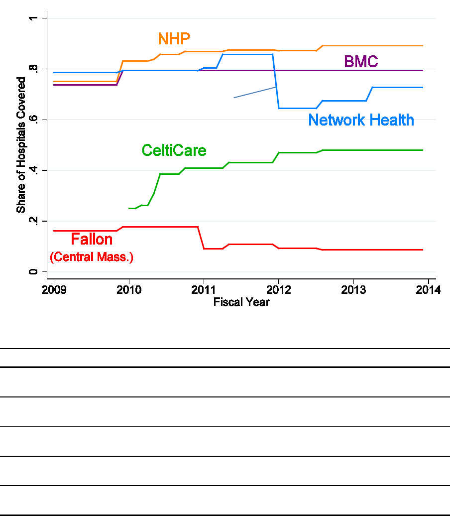
49
Figure 1. Hospital Network Coverage in Exchange Plans
NOTE: The graph shows the shares of Massachusetts hospitals covered by each CommCare plan, where shares are
weighted by hospital bed size in 2011. The table shows coverage of the Partners hospitals, separately for the two star
academic medical centers – Mass. General Hospital (MGH) and Brigham & Women’s Hospital – and for the
number covered among the five Partners community hospitals.
Plan Hospitals 2009 2010 2011 2012 2013
2014 (ACA)
MGH & Brigham No No No No No No
Others 2/5 1/5 1/5 1/5 1/5 0/5
MGH & Brigham Yes Yes Yes No No No
Others 5/5 5/5 5/5 2/5 2/5 0/5
MGH & Brigham Yes Yes Yes Yes Yes Yes
Others 2/5 4/5 4/5 4/5 5/5 5/5
MGH & Brigham --- Yes Yes Yes Yes No
Others 3/5 3/5 3/5 3/5 0/5
MGH & Brigham No No No No No No
Others 0/5 0/5 0/5 1/5 0/5 1/5
CeltiCare
(new in 2010)
Fallon
(mainly central MA)
Boston Medical
Center Plan (BMC)
Network Health
Ne ighborhood
Health Plan (NHP)
Coverage of Partners Hospitals
Network Health
drops Partners
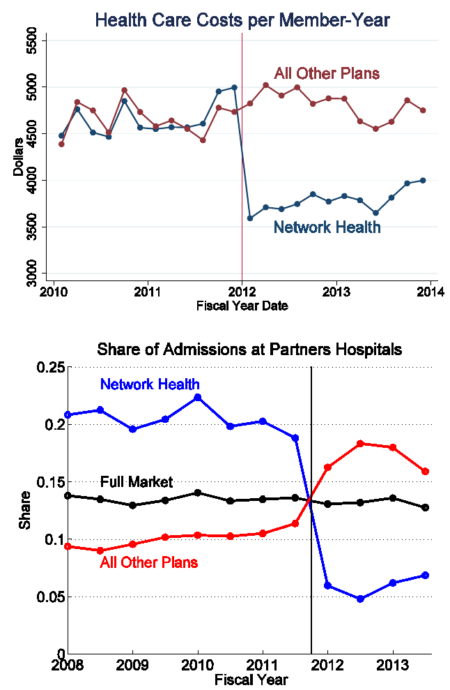
50
Figure 2. Costs and Hospital Use around 2012 Network Health Changes

51
Table 2. Test of Adverse Selection Mechanism: Past Patients at Partners Hospitals
NOTE: The table shows regression results from the unused observables test for adverse selection, as described in
Section 3.1. The bottom section shows raw means of the dependent variables, to show how controlling for risk
affects the between-group differences. The data are at the individual x plan choice instance level for the 2011-2013
period during which I have full risk adjustment data. Cost and hospital use outcomes are defined as averages over
the subsequent year. “Past Patient at Partners Facility” is a dummy for whether an individual has been observed
using a Partners facility for outpatient care prior to the given plan choice instance. The sample excludes new
enrollees into the exchange, for whom past utilization data is not observed. Columns (1)-(4) limit the sample to
plans covering Partners to examine a sample who all have access to the star hospitals. Column (5) limits the sample
to individuals making active plan choices when re-enrolling in the exchange after a gap in coverage. Regressions in
columns (4) and (5) are weighted by the number of months each individual was enrolled during the year. All
standard errors (in parentheses) are clustered at the individual level.
Plan Choice
Share of
Admissions at
Star Hospital
Price per
Admission ($)
Hospitalization
Rate (annual)
Total Cost per
Year ($)
Actively Choose
Plan Covering
Partners
(1) (2) (3) (4) (5)
Past Patient at Partners Facility 0.322** 3,143.0** 0.0039 1,137.3** 0.298**
(0.010) (126.8) (0.0034) (96.3) (0.004)
Control Variables
Risk Score 0.007** 99.2** 0.0953** 4,788.7** -0.004**
(0.002) (22.3) (0.0040) (159.0) (0.001)
Plan x Year x Income Grp FE X
X X X ---
Year x Income Grp FE --- ---
---
--- X
Observations 10,505 10,505 270,198 270,198 172,874
R-Squared
0.184
0.127
0.029 0.117 0.181
De pe nde nt Var. M e ans:
Past Patient at Partners Facility 0.398 14,125 0.111 7,318
0.661
All Others
0.066
10,770 0.072
4,032
0.376
[Difference]
[0.332] [3,355] [0.039] [3,286] [0.285]
** p<0.01, * p<0.05
Dependent Variable:
Hospital Use and Cost (Plans Covering Partners Only)
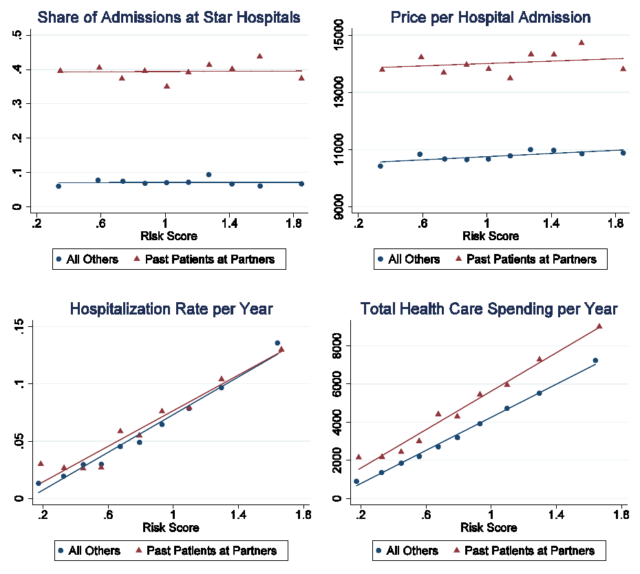
52
Figure 3. Hospital Use and Cost Differences: Past Patients at Partners vs. Others
NOTE: The figures show binned scatter plots, analogous to the adverse selection test regression results in Table 2.
The figures compare outcomes for past Partners patients (in red triangles) to all other enrollees (blue circles), within
bins of medical risk score (the x-axis). The solid lines are best-fit lines for each group. The underlying sample and
data setup are identical to Table 2
. Data are at the individual x plan choice instance level for the 2011-2013 period
during which I have full risk adjustment data. Cost and hospital use outcomes are defined as averages over the
subsequent year. “Past Patients at Partners” is a dummy for whether an individual is observed using a Partners
facility for outpatient care prior to the given plan choice instance. The sample excludes new enrollees in the
exchange (for whom past utilization data is not observed) and is limited to people in plans that cover Partners.
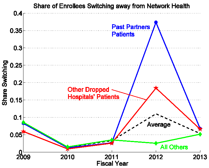
53
Figure 4. Plan Switching after Network Health Dropped Partners in 2012
NOTE: This figure shows the share of enrollees in Network Health plan who switch to another plan at the start of
each fiscal year (when all exchange enrollees are given an opportunity to switch plans). The black dashed lines show
the average switching rate for all enrollees; the colored solid lines decompose this average into subgroups. In most
years, switching rates are quite low, but in 2012, switching spiked after Network Health dropped the star Partners
hospitals and eight other less prestigious hospitals. The graph shows a large switching spike among past patients of
Partners (in blue) and a smaller spike among patients of the other dropped hospitals (in red). There was little change
in switching rates among all other enrollees (in green). These results suggest that many patients are willing to switch
plans to keep access to their regular hospital provider. As I show elsewhere, the past Partners patients were a
particularly high-cost group, so these switching patterns contributed to favorable selection for Network Health when
it dropped Partners.

54
Table 3. Analysis of Costs for Network Health Enrollees, 2011-12
2011 2012
%Δ
2011 2012
%Δ
All Enrollees $4,631 $3,676 -21% $4,439 $3,761 -15% ---
Stayers $3,877 $3,641 -6% $3,807 $3,596 -6% 36,768
Left Plan in 2012
Switched Plans $8,045 [$7,391] --- $6,109 [$5,106] --- 4,640
Exited Market $5,634 --- --- $5,511 --- --- 22,617
Joined Plan in 2012
Switched Plans [$3,391] $3,461 --- [$3,641] $3,706 --- 15,062
Entered Market --- $3,781 --- --- $4,007 --- 51,109
2011 2012
%Δ
2011 2012
%Δ
Stayers
Partners Patients
$6,396 $4,765 -26% $5,662 $3,983 -30% 5,308
All O thers
$3,406 $3,467 2% $3,414 $3,523 3% 31,460
Switched from Network Health in 2012
Partners Patients $9,337 [$8,082] --- $6,853 [$5,259] ---
3,169
All O thers $4,834 [$5,882] --- $4,017 [$4,695] ---
1,471
Exited Market in 2012
Partners Patients $10,280 --- --- $7,770 --- ---
3,150
All O thers $4,865 --- --- $5,002 --- ---
19,467
* Number of enrollees during the relevant year they were enrolled in Network Health.
Enrollee Group
Avg. Costs
Risk-Adjusted Avg. Costs
Group
Size *
Enrollee Group
Avg. Costs
Risk-Adjusted Avg. Costs
Group
Size *
Breakdown by Partners Patient Status

55
Figure 5. Treatment Effects on Per-Member Costs
Panel A: Overall Effects
Panel B: Heterogeneity in Effects
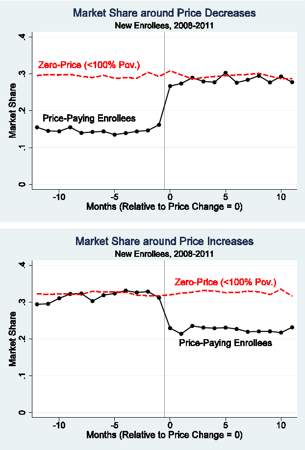
56
Figure 6. Premium Identification and Test of Parallel Trends Assumption
NOTE: These graphs show the source of identification for the premium coefficients in plan demand and test the key
parallel trends assumption for the difference-in-differences approach. Each graph shows average monthly plan
market shares among new enrollees for plans that at time 0 decreased their prices (top figure) or increased their
prices (bottom figure). Each point represents the shares for an independent set of new enrollees. The identification
comes from comparing demand changes for above-poverty price-paying enrollees (for whom premium changes at
time 0) versus below-poverty zero-price enrollees (for whom premiums are unchanged at $0). Consistent with the
parallel trends assumption, trends in shares are flat and parallel for both groups at times other than the premium
change but change sharply for price-payers only at the price change. The sample is limited to fiscal years 2008-
2011. I drop 2007 because above-poverty enrollees did become eligible for the market until mid-way through the
year and 2012+ because below-poverty new enrollees became subject to a limited choice policy that required them
to choose lower-price plans.

57
Table 4. Hospital Demand Estimates
NOTE: The table shows estimates for the multinomial logit hospital choice model described in Section 4.1. The left
columns show a simple model, while the right columns show the full model used for all further analyses. The logit
coefficients shown are interpretable as entering the latent utility function describing hospital choice. Past use
variables are dummies for whether a patient has used each specific hospital at least 60 days before the current
admission. Severity is an estimated summary measure of costs described in Section 5.1
. In addition to the variables
shown, the model includes: distance interacted with exchange region, detailed income group (by 50% of poverty),
and gender; severity interacted with separate dummies for each academic medical center; and five additional
diagnosis x hospital service interactions (circulatory diagnosis interacted with cath lab, interventional cardiology,
and heart surgery services; pregnancy diagnosis x NICU; and musculoskeletal diagnosis x arthritis services).
Coeff. Std. Error Coeff. Std. Error
Distance to Hospital:
Distance in Miles (avg. coeff.) -0.189*** (0.001) -0.144*** (0.001)
Distance^2 (avg. coeff.) 0.0013*** (0.0000) 0.0009*** (1e-5)
Distance Interactions:
x Income > Poverty -0.006*** (0.0006)
x Age / 10 -0.003*** (0.0002)
x Severity Weight -0.002 (0.0011)
x Emergency -0.015*** (0.0006)
Out-of-Network Disutility
Out-of-Network x BMC -1.327*** (0.016) -1.117*** (0.034)
Out-of-Network x CeltiCare -1.464*** (0.058)
Out-of-Network x Fallon -1.583*** (0.059)
Out-of-Network x NHP -0.543*** (0.049)
Out-of-Network x Network -1.011*** (0.036)
Out-of-Network x Emergency 0.010 (0.034)
Past Use of this Hospital (>60 days before)
Inpatient Care 1.417*** (0.020)
Outpatient Care 2.202*** (0.013)
Hospital Characte ristics
Hospital Dummies Yes Yes
Severity x Academic Med. Ctr. (avg). 2.076*** (0.044)
Severity x Teaching Hosp 1.026*** (0.045)
Diagnoses x Hospital Services (largest coeffs.):
Mental: Psych. Services 1.844*** (0.040)
Pregnancy: Obstetrics Services 1.122*** (0.076)
Injury: Level 1 Trauma Center 0.805*** (0.037)
Cancer: Oncology Services 0.704*** (0.084)
Model Statistics:
Pseudo-R^2 (McFadden's) 0.463 0.569
R^2 in Shares (Area-Plan-Yr Level)
0.643 0.742
Num. Choice Instances 74,383 74,383
Std. Errors in parentheses. * = 5% sign., ** = 1% sign., *** = 0.1% sign.
(same for all plans)
VARIABLE
Simple Model
Full Model

58
Table 5. Insurance Plan Demand Estimates
NOTE: This table shows estimates for the multinomial logit plan choice model described in Section 4.3. Premium is
the monthly plan price, which typically varies by $20-60 across plans. (In addition to the interactions shown, the full
model contains interactions with 5-year age groups and gender.) I normalize the average consumer’s premium
coefficient to -1.0, so all other coefficients are interpretable as dollar values. Network utility is the consumer-
specific expected utility measure for a plan’s hospital network, derived in Section 4.2
. Past-used hospitals coverage
is the share of an enrollee’s previously used hospitals that a plan covers, with a separate interaction for the star
Partners hospitals. Switching and inertia are coefficients on a dummy variable for the current plan. The coefficients
are interpretable as “switching costs” in dollars per month; the passive probabilities are the implied share of
enrollees who passively stick with their current plan. The plan brand effects are coefficients on dummies for each
plan. I show average values; the full model contains region-year- and region-income group-specific plan dummies.
VARIABLE Coeff. Std. Error
Premium: Avg. Coeff. (normalized ) -1.000*** (0.025)
x 0-100% Poverty -- Omitted (no prems.) ---
x 100-150% Poverty -1.340*** (0.038)
x 150-200% Poverty -0.935*** (0.024)
x 200-250% Poverty -0.712*** (0.015)
x 250-300% Poverty -0.656*** (0.016)
x Age/5 (average effect) 0.029*** (0.002)
Hospital Ne twork
Network Utility x <100% Poverty 6.355*** (0.885)
Network Utility x 100-150% Poverty 7.371*** (0.939)
Network Utility x 150-200% Poverty 7.453*** (0.962)
Network Utility x 200-250% Poverty 7.736*** (1.270)
Network Utility x 250-300% Poverty 8.541*** (1.878)
Past-Used Hospitals Covered (share) 5.411*** (0.836)
x Past-Used Partners Hospitals 11.631*** (0.773)
Switching and Ine rtia
Passive Prob.
Average Inertia Coefficient 96.810*** (0.230) 94.6%
x Drops Past-Used Hospital (Non-Partners) -29.905*** (1.142) 75.2%
x Drops Past-Used Hospital (Partners) -51.048*** (0.962) 51.8%
Plan Brand Effe cts (ave rage )
BMC HealthNet (normalized) 0.000 ---
CeltiCare -23.088*** (0.890)
Fallon 14.021*** (1.023)
Neighborhood Health Plan -2.199*** (0.251)
Network Health -3.822*** (0.337)
Model Statistics
R^2 in Share (Area-Income-Year)
Model w/ Only Avg. Plan Dummies
No. Choice Instances
No. Unique Individuals
* = 5% sign., ** = 1% sign., *** = 0.1% sign.
0.866
1,588,889
611,455
0.963

59
Table 6. Model Estimates: Relationship between Value and Cost of Partners Coverage
NOTE: This table shows the estimated model’s implication for the relationship between enrollees’ costs and their
value coverage of the star Partners hospitals – the key relationship driving adverse selection. Consumers are sorted
into percentiles of Partners value, and each row shows average values and costs for people in the relevant
percentiles. All values and costs are calculated for current enrollees in 2012 based on the value and cost if Partners
were added to Network Health plan’s network. Value of Partners is defined as the extra plan utility (excluding
switching costs) if Partners is covered, divided the marginal utility of money – based on plan utility estimates shown
in Table 4. Because I cannot estimate marginal utilities for below-poverty enrollees, they are excluded. Costs are
defined using the estimated cost function without Partners covered (columns 2-3) and with it covered (columns 4-7),
both based on the plan cost model in Section 5.3. Column 7 subtracts from the increase in cost an estimate of how
much of these higher costs are funding higher markups for Partners. The table shows that most enrollees value
Partners coverage little, but the top 10-20% values Partners substantially. The table also decomposes two different
reasons people with high values for Partners are high-cost. First, they have higher risk adjusted costs even if Partners
is not covered, which suggests they are unobservably sicker. Second, they have a larger increase in costs when
Partners is covered (column 5) because they use Partners hospitals more often.
Unadjusted
Cost
Risk Adj.
Cost
Risk Adj.
Cost
ΔCost
%Δ
ΔCost - Partners
Hospital Mkup.
(1)
(2) (3)
(4)
(5)
(6) (7)
0-50%
$0.5 $300.0
$301.2
$309.2 $8.0
2.7% $7.0
50-70% $2.2
$269.6
$294.5
$308.6 $14.0
5.2%
$10.6
70-79%
$4.3 $264.3
$292.7
$310.8
$18.1 6.8%
$12.4
80-89%
$8.8
$300.1
$311.8 $335.3
$23.5
7.8%
$14.0
90-95% $23.6
$455.7 $360.4
$398.3 $37.9
8.3% $21.1
96-100% $46.8
$482.3
$340.1 $388.6
$48.5 10.0%
$23.3
Average
$5.7
$308.8 $305.6 $321.2
$15.6
5.0% $10.6
Consumer Value of
Partners Covg.
Costs to Insurer (per month)
Percentiles
Avg. Value
($/month)
Not Covering Partners
Covering Partners

60
Table 7. Simulation Results
NOTE: These tables show equilibrium results for the insurance market simulations described in Section 7.1. In the
game, insurers first simultaneously choose whether or not to cover the Partners hospitals (holding fixed other
hospital coverage) and then simultaneously choose their plan’s price. The tables show their equilibrium choices of
Partners coverage and price. Panel A shows simulations using the Massachusetts exchange’s actual enrollee
population and policies for 2011 – including required minimum and maximum prices – and compares simulated
coverage and prices to the observed values. I do this comparison only for 2011 because of complications with
analyzing other years. As discussed in Section 7.1, the model matches prices well but predicts even more dropping
of Partners than actually occurred (although Network Health dropped Partners the following year). Panel B conducts
simulations with a population and policies closer to those in the ACA exchanges. Specifically, I exclude enrollees
below poverty (who get Medicaid in the ACA), set subsidies as a flat amount for all plans (versus Massachusetts’
higher subsidies for higher-price plans), and do not impose minimum and maximum prices. In these simulations, no
insurer chooses to cover Partners partly because doing so attracts enrollees with high risk-adjusted costs and
therefore lowers profits.
Source Year
Variable BMC
Fallon
Network Hlth NHP CeltiC are
Observed 2011
Partners Covg. No
No Yes Yes
Yes
Price* $424.6
$425.7 $422.6
$425.7
$404.9
Simulated 2011 Partners Covg. No
No
No No Yes
Price* $425.7 $425.7
$425.7 $425.7
$404.9
* Exchange imposed maximum price of $425.7 and minimum price of $404.9
Source Year
Variable BMC
Fallon Network Hlth NHP CeltiCare
Simulated 2011
Partners Covg. No No No
No No
Price $407.2
$409.3 $389.4 $402.5 $318.8
Simulated
2012 Partners Covg.
No No No No
No
Price $427.5 $464.5 $371.0 $417.6
$365.0
Simulated
2013 Partners Covg. No No
No No
No
Price $437.2 $476.8 $432.9 $461.8
$419.4
Insurance Plan
Insurance Plan
Panel A: Mass. Exchange Population & Policies (2011)
Equilibrium Simulation Results
Panel B: ACA-Like Population & Policies

61
Table 8. Counterfactual Policy Simulations
NOTE: This table shows results of simulations of counterfactual policies to address the adverse selection, as
discussed in Section 7.3. The top table shows simulations that modify risk adjustment by over-paying by the listed
“over-adjustment factor” for people with above-average risk scores (and under-paying by the same factor for below-
average risks). The bottom table shows simulations with “marginal subsidies” that narrow price differences across
plans by the listed marginal subsidy rate. All simulations are for the ACA-like population and policies in 2012, so
the baseline results (in the top row of each table) are the same as the 2012 equilibrium in Table 6. Each table lists
which plans cover Partners, the minimum plan price, and average price of all other plans. They also list welfare
statistics in units of dollars per member-month: the change in consumer surplus (with the baseline normalized to $0),
insurer profit, Partners’ net inpatient hospital revenue, and government subsidy costs. The final columns show the
change in social surplus, with an excess government cost of funds (ECF) of either 0 or 0.3. The latter values each $1
of government subsidies as incurring a social cost of $1.3 because of the excess burden of tax financing.
ECF = 0
ECF=0.3
None
None
$365.0 $420.1
$0.0 $26.5
$0.6
$322.7 $0.0
$0.0
25% None
$374.5
$420.9 $4.1
$30.0 $0.6
$330.7
-$0.4 -$2.8
50%
NHP Only $381.3
$426.4 $5.4
$33.4
$1.7 $337.1
-$1.0
-$5.3
Plan Statistics
Avg. Price
Other Plans
Ove r-
Adjus tment
Factor
Risk Adjustment
We lfare Analys is (pe r me mbe r-month)
Covering
Partners
Minimum
P ric e
ΔCons.
Surplus
Insurer
Profit
Partners
Net Rev.
Govt.
Costs
ΔSocial Surplus
ECF = 0
ECF=0.3
None None $365.0 $420.1 $0.0 $26.5 $0.6 $322.7 $0.0 $0.0
15% None $368.8 $427.6 $0.7 $33.4 $0.6 $331.1 -$0.8 -$3.3
25% BMC Only $372.1 $435.9 $0.7 $39.5 $1.0 $338.8 -$1.9 -$6.8
50% BMC + NHP $384.5 $469.4 $2.5 $65.5 $2.4 $370.2 -$4.1 -$18.4
Plan Statistics
Avg. Price
Other Plans
Marginal
Subsidy
Rate
Marginal Subsidies
We lfare Analys is (pe r me mbe r-month)
Covering
Partners
Minimum
P ric e
ΔCons.
Surplus
Insurer
Profit
Partners
Net Rev.
Govt.
Costs
ΔSocial Surplus

62
Appendix A. Sample Summary Statistics
Appendix Table A.1
Mean Mean Std. Dev.
No. of Hospitalizations 74,383 Distance: C hosen Hosp. (miles)
14.1 16.3
Age 44.6
All Hospitals (miles)
48.4 25.9
Male 49% Hospital Category
Emergency Department
56%
Academic Med. Ctr. 29% ---
Diagnoses Mental Illness
16.7% Teaching Hospital 19% ---
Digestive
13.5% All O thers
52% ---
Circulatory 12.6% Partners Hospital 14%
---
Injury / Poisoning 7.1% Out-of-Network 8%
---
Respiratory 7.0%
Past Used Hospital (>60 days before)
Cancer
6.4% Any Use
54% ---
Endocrine / Metabolic 6.0% Inpatient Use
19% ---
Musculoskeletal 5.6% Outpatient Use
51% ---
Genitourinary 5.1%
Total Cost to Insurer $11,369 $15,711
Pregnancy / Childbirth 5.0% Price (estimated)
$10,981 $4,112
All Others 14.9% Patient Severity (estimated) 1.000
0.310
Hospital Choice Sample
Patient Characteristics
Chosen Hospital Statistics
Variable
Variable
Mean
Std. Dev. Mean Std. Dev.
No. of Enrollees
611,455 --- No. of Choice Instances 1,588,889 ---
Age 39.6 13.8
Insurer Price $380.7 $69.5
Male 46.5% --- C ons. Premium: Below Poverty $0.0
$0.0
Income: <100% Poverty 47.1%
--- Above Poverty $47.3 $45.7
100-200% Poverty 39.6% --- Costs per Month: Total
$371.5 $1,480
200-300% Poverty 13.3% ---
Hospital Inpatient $81.5 $1,048
Past Hospital User 44.3% ---
Non-Inpatient $290.0 $873
Partners Hospitals 7.4% --- Current Enr: Non-Switching 95.8% ---
O ther Hospitals 40.3% --- Market Shares: BMC 35.5% ---
Risk Adjustment Score 0.99 0.90
Network Health 34.7% ---
Choice Type: New Enrollee
29.5% --- NHP 19.2% ---
Re- Enrollee 13.5% --- C eltiC are 6.9% ---
Current Enrollee 57.1% --- F allon 3.8% ---
Plan Choice Sample
Variable
Variable
Enrollee Characteristics
Plan Choice Statistics

63
Appendix B. Robustness Tests for Reduced Form Analysis
Appendix Table B.1
Baseline
Regression
Sample: Dx-
Based Risk
Adj. Only
Sample:
Re-Enrollees
O nly
Past Doctor
Visits O nly
Other Past
Hospital Use
Controls
(1) (2) (3) (4) (5)
Past Patient at Partners 1,137.3** 908.2** 1,067.0** 1,304.6** 915.4**
(96.3) (108.0) (162.8) (160.0) (93.5)
Other Past Use Variables:
Any Academic Med. Ctr. 237.1**
(68.9)
Any Hospital 360.6**
(73.7)
Control Variables
Risk Score 4,788.7** 4,561.6** 4,585.6** 4,799.4** 4,752.0**
(159.0) (171.0) (302.4) (159.4) (162.9)
Plan x Year x Income Grp FE X X X X X
Observations 270,198 172,520 71,303 270,198 270,198
R-Squared 0.117 0.132 0.103 0.117 0.117
De pe nde nt Var. Me ans :
Past Patient at Partners 7,318 7,216 6,929 8,088 7,318
All Others 4,032 3,966 4,392 4,321 4,032
[Difference] [3,286] [3,250] [2,537] [3,767] [3,286]
** p<0.01, * p<0.05
Dependent Variable: Total Cost per Year ($)
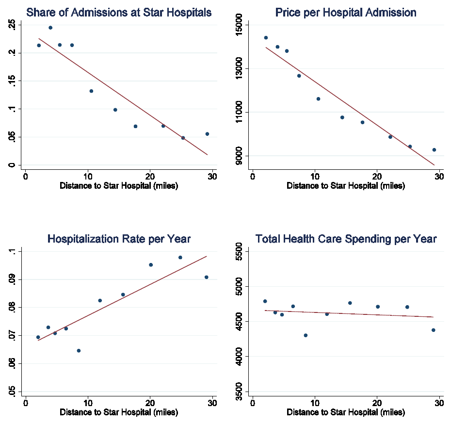
64
Appendix Figure B.1

65
Appendix C. Demand and Cost Model and Estimation Details
C.1. Insurance Plan Demand Estimation Details
I estimate the plan demand model parameters by matching moments that fall into two categories.
First, for plan dummies, I match market shares for the appropriate region/year/income group g. These
market shares uniquely identify plan mean utilities, which in my case are equivalent to the plan
dummies.
89
The formula for these market share moments is:
( ) { } { } ( )
(1)
1
,
,,
1, 1 |
j g it it
N
i jt
G itg yjPryj
θθ
= ∈ ⋅ = − =
∑
where
θ
is the parameter vector,
{ }
1
it
yj=
is an indicator for whether individual i chose plan j at time t,
and
( )
|
it
Pr y j
θ
=
is the predicted choice share from the logit model.
Second, for the coefficients for premium, network utility, and other observed characteristics
(which are interacted with observed enrollee attributes), I match the average values for chosen plans in
the data to those in the model. Specifically, the moments for characteristic
()k
X
(e.g., premium) interacted
with enrollee attribute
()r
Z
(e.g., income) are:
( ) { } ( )
(2) ( ) ( )
1
,
,,
1|
kr
k r ijt it it it
N
i jt
G XZ yjPryj
θθ
= ⋅ = − =
∑
Another way of interpreting these is as matching the covariance between plan characteristics and
household attributes. In the case of observing the full market, these moments are equivalent to the micro
BLP covariance moments. These moments are also equivalent to first-order conditions from the
associated maximum likelihood problem.
Stacking all of the moments into a vector
(
)
G
θ
, the MSM estimator searches for the parameter
θ
that minimizes the weighted sum of squared moments,
( ) ( )
'G WG
θθ
⋅⋅
. Because the system is just-
identified (equal number of parameters and moments), I am able to match the moments exactly, making
the solution invariant to the choice of W. I calculate standard errors using the standard GMM sandwich
formula. To account for the fact that network utility variable is derived from the hospital demand
estimates, I am planning to implement an adjustment following the lecture notes of Pakes (2013).
However, I have not yet implemented this adjustment in the current draft.
89
A difference in my setting from the standard BLP approach is that I treat the plan dummies as parameters, with
associated standard errors, since both they and the characteristics coefficients are estimated from a dataset of the
same size (the full market data). In previous applications including Berry, Levinsohn, and Pakes (2004), the micro
data came from a sample, while the market shares came from aggregate data on the whole market.

66
C.2. Inattention Interpretation of Plan Inertia Coefficients
For current enrollees, I included in the logit demand model a dummy variable for their current
plan, so their full demand utility was:
(
) {
}
Switching Cost / Inertia
ˆ
1
Curr Plan
ijt ijt i ijt
U U Z j CurrPlan
cε
=+ ⋅= +
((((((((
(16)
where
ˆ
ijt
U
is the plan utility for new enrollees (defined in Section 4.3), excluding the
Plan
ijt
ε
. In this
equation,
( )
i
Z
c
is interpreted as a switching cost – an extra utility for the current plan needed to
rationalize the low level of plan switching. The plan demand estimates in Table 4 reports these switching
costs but also an alternate interpretation based on an inattention model. I show here how I derive the
inattention/passive probability reported in Table 4.
Consider a two-step model in which the first step models whether enrollees make an active
choice, and the second step models plan choice conditional on being active. The second step is standard
and follows the logit model for new enrollees (or current enrollees excluding switching cost):
( )
( )
( )
ˆ
exp
|
ˆ
exp
ijt
it
ikt
k
U
Pr y j Active
U
= =
∑
The first step is a reduced form model of being passive:
( )
(
)
( )
( )
( )
,,
,,
,, , ,
ˆ
exp
ˆ
where log exp
ˆ
exp exp
curr
curr
ij t i
it i Active t ikt
k
i j t i i Active t
U
Pr Passive I U
UI
c
c
+
= =
++
∑
Notice that it is the choice probability from a two-choice logit model, where the utility of being passive is
the current plan utility plus a reduced-form inertia coefficient
i
c
(which is different from the switching
cost
c
). The utility of being active is
,,i Active t
I
, which is the inclusive value (or expected utility) from the
second-stage active choice model.
I claim that if
( )
( )
log exp ( ) 1
ii
Z
cc
= −
, the switching cost and inattention models have identical
predictions for choice probabilities. For the current plan, the inattention model predicts a probability that
it is chosen of
( ) (
)
( )
( )
1|
it it it curr
Pr Passive Pr Passive Pr y j Active+− ⋅ =
, which simplifies to:
( )
( )
( )
( )
( ) ( )
,,
,,
ˆ
exp
ˆˆ
exp exp
curr
curr
curr
ij t i
it curr
i j t i ikt
kj
UZ
Pr y j
UZ U
c
c
≠
+
= =
++
∑
This equals the current plan’s choice probability in the switching cost model in (15). Further, the
inattention model’s probability of switching to another plan j is
( )
(
)
( )
1|
it it
Pr Passive Pr y j Active− ⋅=
,
which simplifies to:

67
( )
( )
( )
( ) ( )
,,
,,
ˆ
exp
ˆˆ
exp exp
curr
curr
i jt
it
i j t i ikt
kj
U
Pr y j
UZ U
c
≠
= =
++
∑
which is again equivalent to the choice probability from the switching cost model in (15).
Hence, these two models have equivalent predictions for choice probabilities. The plan demand
results in Table 4 report both the average switching costs
( )
i
Z
c
and the passive probability
( )
it
Pr Passive
, as defined by the equation above.
C.3. Details of Hospital Price Model
As discussed in Section 5.1, I estimate a risk-adjusted hospital price model. Recall that I estimate
a Poisson regression (also known as a generalized linear model with a log link) of the form:
( )
,,,, ,,
| , exp
i j h t a ita ita j h t ita ita
E Payment Diag Z Diag Z
ρ lγ
= ++
For the principal diagnosis (
ita
Diag
), I use the Clinical Classification Software (CCS) dummies defined
by the U.S. government’s Agency for Healthcare Research and Quality. The additional covariates
()
ita
Z
include age, gender, income, and Elixhauser comorbidity dummies for the secondary diagnoses.
I specify a restricted model for
,,jht
ρ
to avoid over-fitting for hospital-insurer-year cells with
small samples. Specifically, I start from the model:
, , , , ( ,) , ( ), ,, ( ,)j h t j h NetwStat h t j Sys h t j t NetwStat h t
ρρ ρ ρ
= ++
The first term,
, , ( ,)j h NetwStat h t
ρ
, is a coefficient on hospital-insurer-network status (i.e., in or out of
network) dummies that is constant across years. I include this term for all cells with at least 50
observations; otherwise, I set it to zero. The second term,
, ( ),j Sys h t
ρ
, is a coefficient on insurer-hospital
system-year dummies for the top six hospital systems. This allows for a separate hospital price paths over
time for each of the largest systems (including Partners). I do not include this term for hospitals in smaller
systems or when the large system is out-of-network, with the exception that I always include these
dummies for Partners regardless of whether it is in-network. The final term,
,, ( ,)j t NetwStat h t
ρ
, is a residual
that allows for a separate effect for each plan, year, and network status. This captures the average insurer-
specific price path for all smaller hospitals not included in one of the six largest systems.
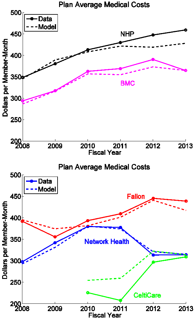
68
Appendix D. Model Fit Tables and Figures
This appendix shows tables and figures that display the model’s ability to match the reduced form
patterns around Network Health’s dropping of the Partners hospitals in 2012, as discussed in Section 5.4.
Appendix Figure D.1. Model Fit for Plan Average Medical Costs
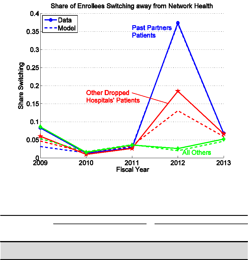
69
Appendix Figure D.2. Plan Switching Patterns
Appendix Table D.1. Cost Changes for Network Health
2011 2012
%Δ
Ris k Adj.
%Δ
2011
2012
%Δ
Ris k Adj.
%Δ
All Enrollees $378
$313 -17% -15% $374
$310 -17% -16%
Stayers (in plan
both years)
$317
$305 -4% -5% $334 $312
-7% -9%
2011 Only Enrollees $476 --- --- $435
--- ---
2012 Only Enrollees
--- $310 --- --- $302 ---
Data
Model
Enrollee Group
Network Health: Average Costs 2011-12
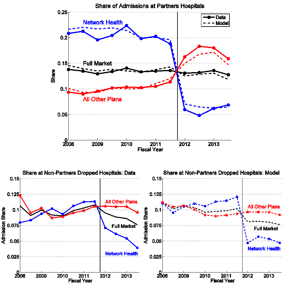
70
Appendix Figure D.3. Admission Shares at Hospitals Dropped by Network Health in 2012
NOTE: These figures show the share of hospital admissions at hospitals that Network Health plan dropped from its
network in 2012. The dashed lines show the model’s prediction for the same statistics. These are calculated holding
fixed each individual’s observed plan, not reassigning plan choices using the plan demand model.
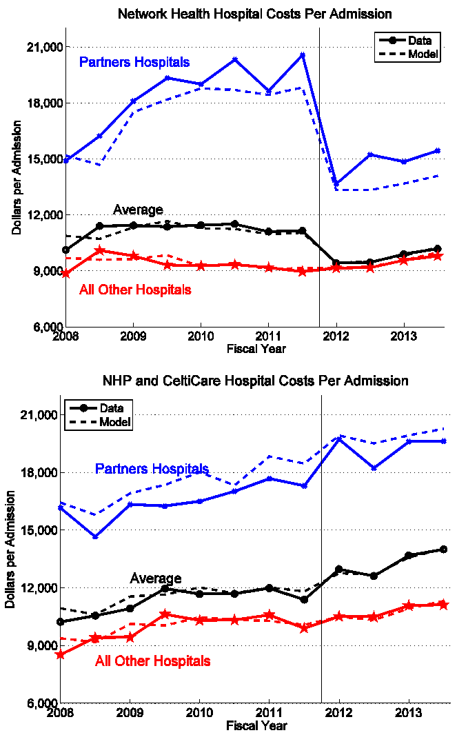
71
Appendix Table D.4. Changes in Cost per Hospital Admission around 2012 Network Changes
NOTE: These figures show average costs per hospital admission for two sets of plans: Network Health (top figure),
which dropped the star Partners hospitals in 2012, and NHP and CeltiCare (bottom figure), which continued to cover
them. The dashed lines show the model’s prediction for the same statistics. These are calculated holding fixed each
individual’s observed plan, not reassigning plan choices using the plan demand model.

72
Appendix E. Simulation Method Details
This appendix details the simple approach I use to incorporate a future profit effect in a static pricing
model for my simulations in Section 7. Note that in a dynamic model, an insurer’s pricing FOC includes a
term capturing the effect of changing today’s price on future profits on consumer i. I model this “future
profit effect” as the product of the change in future demand
( /)
Fut
ij j
DP∂∂
times an expected profit margin
Fut
ij
M
, which is unaffected by today’s price. For the change in future demand, a lower price increases
demand today and therefore increases the number of inertial enrollees in the future. To simplify, I take
future market enrollment
,
()
it k
nMon
+
as given and assume an exogenous, constant inertia probability
h
at each year’s switching choice, which I set at 89%.
90
Given these assumptions:
,
1
Fut
ij ij
k
it k
k
jj
DS
nMon
PP
h
+
≥
∂∂
=⋅⋅
∂∂
∑
(17)
where
/
ij j
SP∂∂
is the effect of price on current year’s choice share.
Finally, I need to specify insurers’ future profit margins. Although imperfect, I simply assume
that insurers expect
Fut
ij
M
to equal current margins at the enrollee level – which assumes that prices and
costs grow in parallel for each enrollee. Notice that I still treat
Fut
ij
M
as a constant in the pricing FOC but
plug in the equilibrium margin (
(
)
*
i j ij j
P cN
j
= −
) for it at the end.
Combining these assumptions and defining the term in parentheses in (16) as
i
nFutMon
, the
pricing FOC for insurer j is:
( )
(
)
( )
0
.
Fut
j ij
Fut
ij
i
jj
ij
i i ij i j ij i i
ii
j
D
M
PP
S
nMon S P c nMon nFutMon
P
π
jj
∂∂
=+⋅
∂∂
∂
=⋅ ⋅+ − + ⋅
∂
∑
∑∑
(18)
Accounting for future profits adds the
i
nFutMon
term to the FOC, which increases the incentive to lower
prices (just like a steeper demand curve). This effect is likely to have a significant impact. Months in the
current year
()
i
nMon
average 6.2, and future months
()
i
nFutMon
average 6.8. So the future profit effect
works like a more than doubling of the demand slope.
90
I use 89% rather than the 95% inertia probability reported in the plan demand estimates based on a rough
correction for unobserved heterogeneity. Looking at re-enrollees (people who leave the market and return later),
people tend to actively choose the same plan as during their prior spell about 55% of the time. For an inertia
probability of
ρ
the overall non-switching probability is
(1 )
Active
j
Pr
ρρ
+− ⋅
. Plugging in
55%
Active
i
Pr =
,
89%
ρ
=
is
required to rationalize a 95% overall non-switching probability.
