
Credit Default Swap –Pricing Theory, Real Data Analysis and Classroom Applications
Using Bloomberg Terminal
Yuan Wen *
Assistant Professor of Finance
State University of New York at New Paltz
1 Hawk Drive, New Paltz, NY 12561
Email: [email protected]
Tel: 845-257-2926
Jacob Kinsella
MBA Candidate
State University of New York at New Paltz
Email: [email protected]
*Primary Author
Abstract
The valuation of Credit default swaps (CDS) is intrinsically difficult given the confounding
effects of the default probability, loss amount, recovery rate and timing of default. CDS pricing
models contain high-level mathematics and statistics that are challenging for most undergraduate
and MBA students. We introduce the basic CDS functions in the Bloomberg Terminal, aiming to
help the students visualize the complicated concept of CDS. Furthermore, we use real data
extracted from the Bloomberg terminal to illustrate the CDS pricing model of Hull and White
(2000). Our paper can be used in an upper-division undergraduate Finance class or an MBA
class.
1
I. Introduction
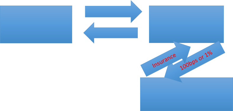
A credit default swap (CDS) is a derivatives instrument that provides insurance against the risk
of a default by a particular company. This contract generally includes three parties: first the
issuer of the debt security, second the buyer of the debt security, and then the third party, which
is usually an insurance company or a large bank. The third party will sell a CDS to the buyer of
the debt security. The CDS offers insurance to the buyer of the debt security in case the issuer is
no longer able to pay. In the case of a default, the seller of the CDS is obligated to buy the debt
security for its face value from the buyer of the CDS.
An example of a CDS will help illustrate how the cash flows work. In this example,
Company X is issuing a 10-year, 8% bond with a $10 million par value. Company Y has excess
liquid funds, which are earning no interest at this time, and so they decide to buy Company X’s
bond. Company X is given a rating of BB by a credit rating agency, and so Company Y thinks
that it would be beneficial to seek a credit default swap from New National Bank. The contract is
written up and states that for the entire duration of the bonds life, Company Y will pay 1% of the
face value to the bank. In return, the bank will offer insurance against Company X defaulting on
their bond payment. The cash flows are illustrated below.
Company X (Bond
issuer)
8%/Year + Par
$10 Million
Company Y (Bond
purchaser)
New National Bank

2
The notional value of a CDS refers to the face value of the underlying security. When
looking at the premium that is paid by the buyer of the CDS to the seller, this amount is
expressed as a proportion of the notional value of the contract in basis points. Gross notional
value refers to the total amount of outstanding credit default swaps.
CDS can be written on loans or bonds. For simplicity, we only examine CDS written on
bonds. If the reference entity (bond issuer) defaults at time t (t<=T, where T is the maturity
date), the CDS buyer will get a payment from the seller. This payment is referred to as the payoff
from the CDS. The payoff from a CDS is usually different from the amount of the debt because
the recovery rate is non- zero in most cases. When a bond defaults, bondholders will typically get
part of their investment back from the liquidation of the issuer’s assets. According to Moody’s
ultimate recovery database, the mean and median recovery rates for bonds are 37 percent and 24
percent, respectively
1
. The payoff from a CDS in the event of a default is usually equal to the
face value of the bond minus its market value just after t, where the market value just after t is
equal to recovery rate × (face value of the bond +accrued interest) (Hull and White,2000).
II. Basic CDS Functions in Bloomberg Terminal
Real-time and historical information about CDS can be extracted from the Bloomberg
terminal. We use Ford Motor Co. as an example. By typing in “RELS” under Ford Motor Co.,
we can find all the non-equity securities related to the company. By selecting “Par CDS spread”,
we will find CDS contracts written on Ford bonds of various maturities.
1
https://www.moodys.com/sites/products/DefaultResearch/2006600000428092.pdf
3
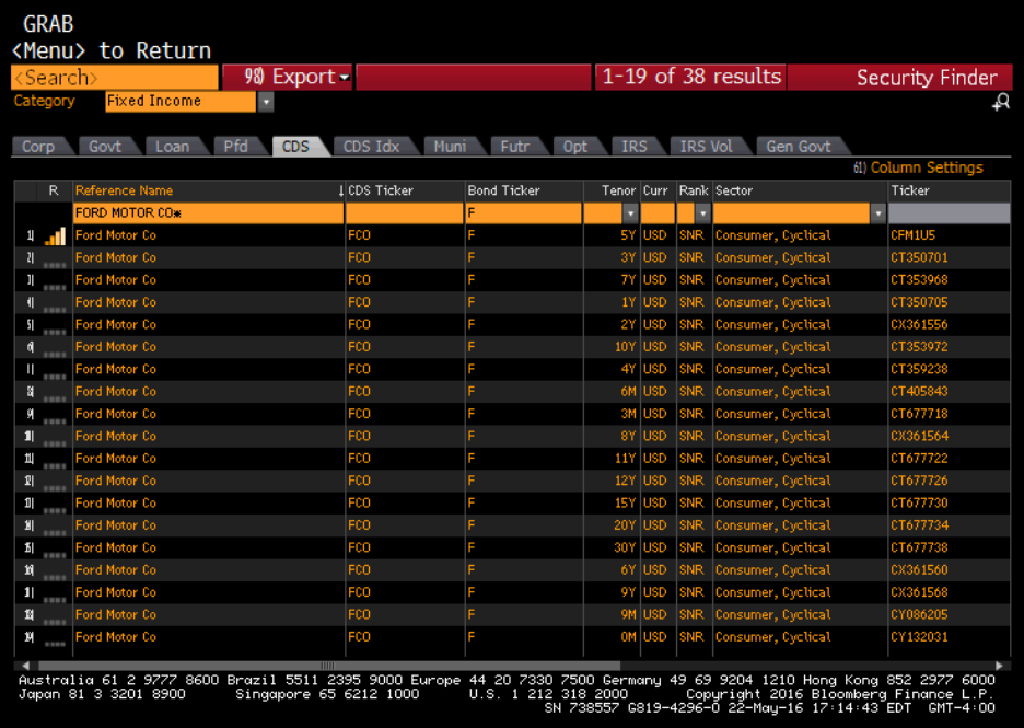
Figure 1
Figure 1 is a snapshot of the Bloomberg window for “Par CDS spread”. The window
shows that Ford has multiple CDS contracts outstanding, each based on a different bond. We
choose the CDS contract based on the 5-year senior bond (the first one in the list) for illustration
as this is the most liquid CDS contract. Subsequently, type in “HP” to find the historical prices
for this CDS contract.
4
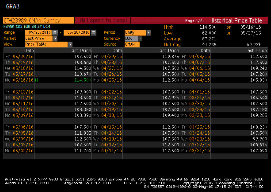
Figure 2
Figure 2 shows the output window for the function “HP” (historical price). The default
price shown in the window is last price. We can change the variable displayed to bid price or ask
price using the drop down box of the “Market” field. The price is also known as CDS spread,
which is usually expressed as a proportion of the notional value in basis points. Normally, the
buyer of the CDS makes a payment to the seller every quarter. If default occurs before the
maturity date of the CDS, the buyer will have to pay the seller the “accrued payment” for the
period that starts at last payment date and ends at the day when default occurs. After that, no
further payment would be required. The CDS-Bond basis is the difference between CDS spread
and bond yield spread (bond yield spread= bond yield-risk free rate).
5
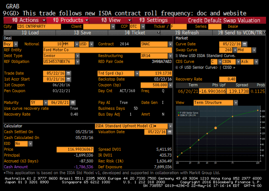
Figure 3
Another powerful function of the Bloomberg terminal is CDSW, the CDS pricing tool of
Bloomberg. Figure 3 shows the output window for CDSW. The Bloomberg CDS model prices a
credit default swap as a function of its schedule, deal spread, notional value, CDS curve and
yield curve. The key assumptions employed in the Bloomberg model include: constant recovery
as a fraction of par, piecewise constant risk neutral hazard rates, and default events being
statistically independent of changes in the default-free yield curve. Figure 3 shows the price of a
Ford Motor CDS calculated using the Bloomberg CDS model. You can change the reference
entity (bond issuer) and bond type in the “REF Entity” field and the “Debt Type” field
respectively. You can then enter today’s date in the “Trade Date” field if you were to trade
6
today and the last day of your planned holding period in the “Maturity Date” field. The default
recovery rate is set to be 40%. However, you can change it to any other rate in the “Recovery
Rate” field. As shown in the “Price” field, the CDS price calculated using the Bloomberg model
is 116.99 basis points based on a $10 million notional value.
III. Pricing
The basic idea of CDS pricing is that the present value of all CDS premium payments should
equal the present value of the expected payoff from the CDS for the NPV to be 0 for both parties
of the contract (resulting in each party being equally well off).
1. The Hull &White Valuation Model:
In this section, we introduce the most cited CDS valuation model, the Hull &White model. In
this model, the price for a $1 notional value CDS are calculated as follows:
π, the risk-neutral probability of no default during the life of the swap (that matures at T) is
calculated as:
π = 1-
(1)
where q(t) is the risk-neutral default probability density at time t and T is the maturity date of the
CDS.
If no default occurs for the life of the CDS, the present value of the payments is ω μ(T),
where ω is the total payment per year made by CDS buyer and μ(t) is the present value of
payments at the rate of $1 per year on payment dates between time zero and time t. If, however,
a default occurs prior to T, say at time t, the present value of the payments will be

7
ω [μ(t)+e(t)] where e(t) is the present value of an accrual payment at time t equal to t-t* (t* is the
payment date immediately preceding time t). Therefore, the expected present value of the
payments is given by
Next, we need to find the present value of expected payoff from the CDS. For a $1
notional value, the payoff from the CDS is 1-
[1+A(t)] = 1-
-
*A(t), where
is the expected
recovery rate on the reference obligation in a risk-neutral world and A(t) is the accrued interest
on the reference obligation at time t as a percent of face/notional value. The present value of the
expected payoff is:
(3)
where υ(t) is the present value of $1 received at time t.
For the PV of the expected payoff to be the same as the PV of the expected value of the
payments, (2) must equal (3). The value of ω that makes (2) equal (3) is the CDS spread.
Therefore, we derive the CDS spread as:
CDS spread =
(4)
2. Finding the Default Rate
The risk neutral default probability q(t) is the key input to most CDS pricing models. This
section illustrates the calculation of the risk neutral default probability for Ford Motor Co. For
instructors who are using this paper in the classroom, you can assign the following project
to the students:
8
Please collect data for the bonds of a company of your choice and calculate the risk-
neutral default probability following the Ford. Motor Co. example as detailed below, assuming
that you are interested in a 5-year CDS based on senior bonds.
Hull and White (2000) suggest that the risk-neutral default probability for a bond can be
inferred from the difference between the bond yield and a default-free bond yield (i.e. Treasury
bond yield). In this section, we use data from Bloomberg Terminal to estimate the risk neutral
default probability q(t).
First, we use a simplified case where the recovery rate is zero to illustrate the basic idea.
Assume the continuously compounded yield on a 10-year zero-coupon treasury bond and that on
a 10-year zero-coupon corporate bond are given as follows:
Yield on zero-coupon Treasury bond
Yield on zero-coupon corporate bond
3.3%
3.9%
The present values of the two bonds are $1000e
-0.033×10
=$718.92, and $1000e
-
0.039×10
=$677.06. The difference of $41.86 ($718.92-$677.06=$41.86) is the present value of the
cost of default. Given a default probability of p, the present value of the expected loss is
1000×p× e
-0.033*10
, which should be the same as $41.86. Therefore,
1000pe
-0.033*10
=41.86
Solving the equation for p, we find p= 0.058226.
If a company has multiple bonds with different maturity dates outstanding, we need to
incorporate all the bonds in estimating the default probability. Hull and White suggest that the
risk neutral default probability at time j (j is the maturity date of the j
th
bond) is given by
p
j
=
(5)
9
where P
j
is the default probability at t
j
, B
j
is the price of the j
th
corporate bond and Gj is the price
of the Treasury bond promising the same cash flows as the j
th
corporate bond. α
ij
is the present
value of the loss in the event of default on the j
th
bond at time t
i
, relative to the value “the bond
would have if there were no possibility of default”. α
ij
is given by :
α
ij
= υ (t
i
) [F
j
(t
i
) – R
j
(t
i
)C
j
(t
i
)] (6)
where υ (t) is the present value of $1 received at time t with certainty, F
j
(t) is the forward price
of the j
th
bond for a forward contract maturing at time t assuming the bond is default–free (t<t
j
),
R
j
(t) is the recovery rate for holders of the j
th
bond in the event of a default at time t (t<t
j
), and
C
j
(t) is the claim made by holders of the j
th
bond if there is a default at time t (t<t
j
).
From the Bloomberg terminal, we can find all the bonds outstanding, their maturity dates,
price, yield and rating. We find 16 bonds outstanding for Ford. Since we are only interested in
the 5-year CDS, we identify the bonds whose time to maturity is the closest to 5 years (referred
to as “Bond A”) and the bonds that have a maturity date earlier than that of Bond A. All the
bonds included in our analysis are shown in Table 1.
[Insert Table 1 here]
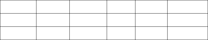
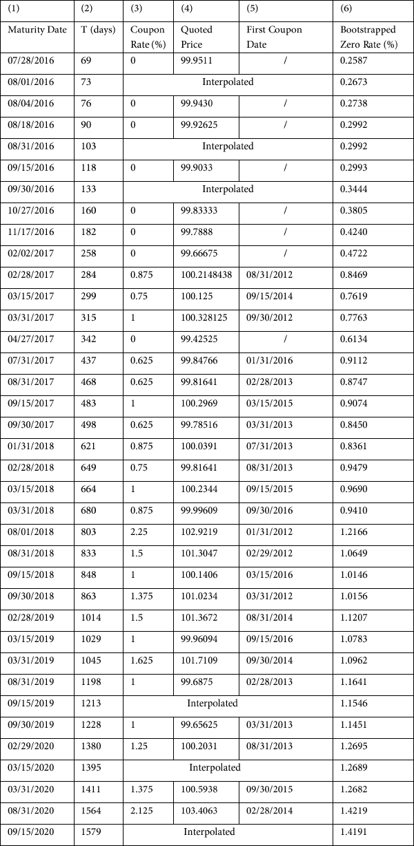
We also use Bloomberg terminal to find the treasury bonds outstanding, their maturity
dates, coupons, quoted prices and yields. Information regarding treasury bonds is included in
Table 2, columns 1-5. Column 6 reports the zero-coupon rates we bootstrapped from the
information given in columns 1-5.
[Insert Table 2 here]
The 3-month Treasury bill that expires on 08/18/2016 has a price of 99.92625 per $100
face value. To find its continuously compounded yield, we use the formula: FV=PV × e
rt
. By
plugging in the values for PV and FV, we’ll find 100 = 99.92625×e
(90/365)r
. Solving the equation,
10
we find that r, the continuously compounded yield equals 0.2992%. Using the same methods,
we find the continuously compounded yields for the 6-month (maturing on 11/17/2016) and 1-
year (maturing on 04/27/2017) treasury bills are 0.4240% and 0.6134%, respectively.
The coupon bond that matures 1.5 years from now (10/31/2017) is priced at $99.92188.
To find the zero-coupon rate for 10/31/2017, we need to look at the coupon payments that will
occur by the maturity date. Based on the first coupon date, we know that future payments are
scheduled as follows:
10/31/2016 (164 days from today): $0.375 ($100*0.75%/2=$0.375)
04/30/2017 (345 days from today): $0.375
10/31/2017 (529 days from today): $0.375 + $100= $100.375.
Given the quoted price of $99.92188 and the zero coupon rates for 10/31/2016 and 04/30/2017,
we know that
0.375e
-(164/365)*0.003805
+ 0.375e
-(345/365)*0.006134
+ 100.375e
-(529/365)*r
=99.92188 (7)
Solving equation (7)
2
for r, we find r=0.8301%, which is the zero-coupon rate for 10/31/2017.
We do the same thing for all other treasury bonds and find the zero-coupon yields for all other
periods. If bonds maturing on a desired date are not available, we use interpolation to find the
zero-coupon rate for that date. For example,
The zero-coupon rate for Aug. 18, 2016 is 0.2992% and that for Sep. 15 2016 is
0.2993%, we can interpolate the rates to find the zero-coupon rate for Aug 31, 2016 as follows:
0.2992% +
× (0.2993%-0.2992%) =0.2992%
2

11
Our next step is to examine the characteristics of the two bonds issued by Ford. The first
bond will make coupon payments on dates listed in Column 1 of Panel 1, Table 3, with
08/01/2018 being the maturity date when the face value ($100) is paid. The coupon dates for the
second bond are listed in Column 1 of Panel 2, Table 3. G
j
, the present value of the Treasury
bond that has the same cash flows as the j
th
bond is calculate by discounting all the coupon
payments in column 2 using the relevant zero-coupon rate in Table 2.
[Insert Table 3 here]
Using the method described above, we find G1= $113.4293 and G2 = $141.1141 (See
Panels 1 and 2, Table 3). Based on equation (6): α
ij
= υ (t
i
)[F
j
(t
i
) – R
j
(t
i
)C
j
(t
i
)], we find α
11,
the
PV of loss from a default on the 1
st
bond at the maturity date of the 1
st
bond = (103.25-
0.4*103.25) * e
-0.012166*803/365
= 60.3139. It follows that P
1
= (G
1
-B
1
)/ α
11
= (113.4293-108.125)/
60.3139=0.08794.
To find α
12,
the PV of loss from a default on the 2nd bond at the maturity date of the 1
st
bond, we need to find C
2
(t
1
) –claim amount and F
2
(t
1
)-forward price of the second bond on the
maturity date of the first bond (08/01/2018), assuming the bond is default-free:
C
2
(t
1
) = 100+ [(4.6075*6) + 4.6075*(139/ 184 )] = $131.12567.
Hull and White (2000) and Jarrow and Turnbull (1995) assume that the bondholder
claims the non-default value of the bond in the event of a default, which implies that C
j
(t) = F
j
(t).
Therefore, we can assume that F
2
(t
1
) is the same as C
2
(t
1
). Consequently, α
12
= (131.12567-
0.4*131.12567) * e
-0.012166*803/365
= 76.5976, C
2
(t
2
) = 100+ 4.6075 = 104.6075, α
22
= (104.6075-
0.4*104.6075) *e
-0.015286*1944/365
= 57.8571
p
2 =
=
= 0.08592
With p
1
and p
2
, we can find the cumulative default probability on 09/15/2021 as follows:
12
Cumulative default probability
2
= 1- [(1-0.08794)*(1-0.08592)] = 0.166304. Using the method
described above, we can find the default probability and cumulative default probability for any
given maturity dates.
IV. Further Classroom Application: Examine Liquidity of Single-name CDS Market
Since its introduction in 1997, the CDS market had been increasing rapidly until 2006-
2007. At the end of 2009, the total notional value of credit default swaps was $30.4 trillion,
which was an astronomical decrease from a total notional value of around $41 trillion in 2008
and $60 trillion in 2007. The decrease in liquidity was caused by a combination of factors
including new regulations and changing investor risk-taking preferences. Firstly, the Dodd-
Frank Act passed in 2010 made holding swaps more expensive for banks. As a result, many big
banks retreated from the CDS market. Secondly, a prolonged decline in volatility caused by a
loose monetary policy since 2008 made buyers less apt to purchase protection.
As part of the assignment, the instructors can ask the student to do the following:
Collect the bid price and ask price for the CDS of your choice from 2002 to 2016, calculate the
bid-ask spread and examine the change in bid-ask spread (a proxy for liquidity) during this
period.
Liquidity is measured as the bid-ask spread scaled by the midpoint of the bid price and
ask price. Bid-ask spread is widely used as a measure of liquidity for CDS (Pu and Zhang, 2012).
Volume, which is another popular measure of liquidity, is not publicly available because CDS
Date
Default Probability
(R=40%)
Cumulative Default Probability
(R=40%)
08/01/2018
0.08794
0.08794
09/15/2021
0.08592
0.166304
13
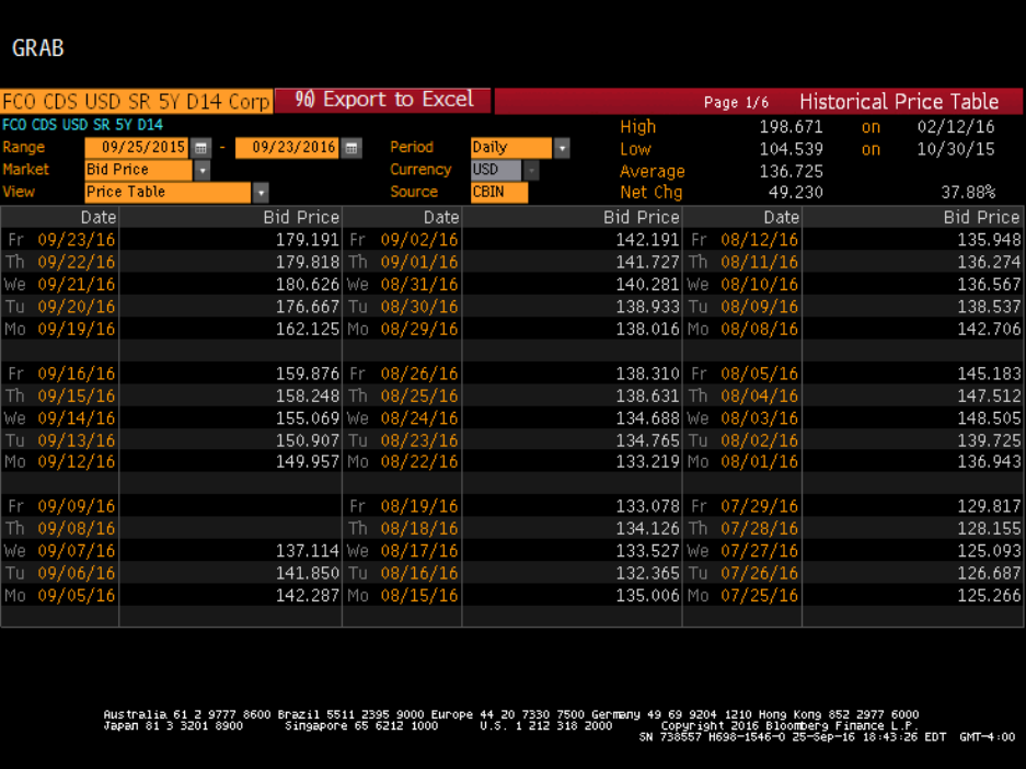
are traded over-the-counter. To find the bid-ask spread, you can follow the instructions under
Figure 1 and Figure 2 (Ford US Equity- RELS – PAR CDS Spreads-HP). The output window
for bid price is shown in Figure 4. You can set the date range to be from 01/01/2002 to the
current date in the “Range” field and then click on “Export to Excel”.
Figure 4
Table 4 reports the annual mean and median liquidity of the CDS market for Ford Motor
Co. from 2002 to 2016. We can see that liquidity peaked in 2006 and then tumbled in 2008. Year
2016 sees the lowest liquidity since 2002.
14
[Insert Table 4 here]
Reference:
Hull, J. C. and A. White, 2000. Valuing Credit Default Swaps I: No Counterparty Default Risk.
Journal of Derivatives 8 (1), p29-40
Jarrow, R.A. and S. Turnbull, 1995. Pricing Options on Derivative Securities Subject to Credit
Risk. Journal of Finance 50 (1), 53-85
Pu, X. and J. Zhang, 2012. Sovereign CDS Spreads, Volatility, and Liquidity: Evidence from
2010 German Short Sale Ban. Financial Review 47(1), p171-197.
15
Table 1: Bonds Outstanding for Ford Motor Co. on 05/20/2016
Coupon (%)
Maturity
Rating
Ask Price
Yield (%)
1st Coupon
Date
6.5
08/01/2018
BBB-
108.125
2.643325
02/01/1999
9.215
09/15/2021
BBB-
129.417
3.14915
09/15/1998
16
Table 2: Treasury Bonds and Bootstrapped Zero-coupon Rates on 05/20/2016
17

18
Table 3: Calculating G
1
and G
2
Panel 1: G
1
: For Bond Maturing on 08/01/2018
Panel 2: G
2
: For Bond Maturing on 09/15/2021
(1)
(2)
(3)
(4)
(5)
Date
Cash
flow
Zero-
coupon
rate
Days
Discounted
cash flow
(2)*e
-(3)*(4)/365
08/01/2016
3.25
0.2673%
73
3.248263
02/01/2017
3.25
0.4722%
257
3.239212
08/01/2017
3.25
0.9112%
438
3.214657
02/01/2018
3.25
0.8361%
622
3.204022
08/01/2018
103.25
1.2166%
803
100.5231
G1 (sum of (5)) = 113.4293
(1)
(2)
(3)
(4)
(5)
Date
Cash
flow
Zero-
coupon
rate
Days
Discounted
cash flow
(2)*e
-(3)*(4)/365
09/15/2016
4.6075
0.2993%
118
4.6030
03/15/2017
4.6075
0.7619%
299
4.5788
09/15/2017
4.6075
0.9074%
483
4.5525
03/15/2018
4.6075
0.9690%
664
4.5270
09/15/2018
4.6075
1.0146%
848
4.5002
03/15/2019
4.6075
1.0783%
1029
4.4695
09/15/2019
4.6075
1.1546%
1213
4.4341
03/15/2020
4.6075
1.2689%
1395
4.3894
09/15/2020
4.6075
1.4191%
1579
4.3331
03/15/2021
4.6075
1.4425%
1760
4.2979
09/15/2021
104.6075
1.5286%
1944
96.4285
G2 (sum of (5)) = 141.1141
19
Table 4: Liquidity of the CDS Market for Ford Motor Co.
Year
Mean
Median
2002
0.0377
0.0387
2003
0.0611
0.0480
2004
0.0273
0.0261
2005
0.0177
0.0163
2006
0.0092
0.0087
2007
0.0117
0.0096
2008
0.0478
0.0476
2009
0.0545
0.0548
2010
0.0503
0.0512
2011
0.0341
0.0282
2012
0.0307
0.0286
2013
0.0477
0.0473
2014
0.0553
0.0546
2015
0.0558
0.0543
2016
0.0588
0.0600
Appendix I
Table A1: Recovery Rates on Corporate Bonds as a Percentage of Face Value, 1982-2012,
from Moody’s
Class
Average recovery rate (%)
Senior secured bond
51.6%
Senior unsecured bond
37.0%
Senior subordinated bond
30.9%
Subordinated bond
31.5%
Junior subordinated bond
24.7%
