NBER WORKING PAPER SERIES
OWNER INCENTIVES AND PERFORMANCE IN HEALTHCARE:
PRIVATE EQUITY INVESTMENT IN NURSING HOMES
Atul Gupta
Sabrina T. Howell
Constantine Yannelis
Abhinav Gupta
Working Paper 28474
http://www.nber.org/papers/w28474
NATIONAL BUREAU OF ECONOMIC RESEARCH
1050 Massachusetts Avenue
Cambridge, MA 02138
February 2021, revised August 2023
We are grateful to Abby Alpert, Pierre Azoulay, Zack Cooper, Liran Einav, Paul Eliason, Arpit
Gupta, Jarrad Harford, Steve Kaplan, Holger Mueller, Aviv Nevo, Adam Sacarny, Albert Sheen,
Arthur Robin Williams, numerous seminar participants, and two anonymous referees for their
comments and suggestions. Jun Wong, Mei-Lynn Hua, and Sarah Schutz provided excellent
research assistance. A previous version of this paper was titled “Does Private Equity Investment
in Healthcare Benefit Patients: Evidence from Nursing Homes." Funding from the Wharton Mack
Institute and the Laura and John Arnold foundation (Gupta, Yannelis), the Kauffman Foundation
(Howell), and the Fama Miller Center at the University of Chicago (Yannelis) is greatly
appreciated. We gratefully acknowledge funding through National Institute of Aging pilot grant
P01AG005842-31. All remaining errors are our own. The views expressed herein are those of the
authors and do not necessarily reflect the views of the National Bureau of Economic Research.
NBER working papers are circulated for discussion and comment purposes. They have not been
peer-reviewed or been subject to the review by the NBER Board of Directors that accompanies
official NBER publications.
© 2021 by Atul Gupta, Sabrina T. Howell, Constantine Yannelis, and Abhinav Gupta. All rights
reserved. Short sections of text, not to exceed two paragraphs, may be quoted without explicit
permission provided that full credit, including © notice, is given to the source.

Owner Incentives and Performance in Healthcare: Private Equity Investment in Nursing Homes
Atul Gupta, Sabrina T. Howell, Constantine Yannelis, and Abhinav Gupta
NBER Working Paper No. 28474
February 2021, revised August 2023
JEL No. G3,G32,G34,G38,I1,I18
ABSTRACT
Amid an aging population and a growing role for private equity (PE) in elder care, this paper
studies how PE ownership affects U.S. nursing homes using patient-level Medicare data. We
show that PE ownership leads to lower-risk patients and increases mortality. After instrumenting
for the patient-nursing home match, we recover a local average treatment effect on mortality of
11%. Declines in measures of patient well-being, nurse staffing, and compliance with care
standards help to explain the mortality effect. Overall, we conclude that PE has nuanced effects,
with adverse outcomes for a subset of patients.
Atul Gupta
Wharton Health Care Management
3641 Locust Walk, CPC 306
Philadelphia, PA 19104
and NBER
Sabrina T. Howell
NYU Stern School of Business
KMC 9-93
44 West 4th Street
New York, NY 10012
and NBER
Constantine Yannelis
Booth School of Business
University of Chicago
5807 S. Woodlawn Avenue
Chicago, IL 60637
and NBER
Abhinav Gupta
UNC Chapel Hill

1 Introduction
The U.S. population, like that of many advanced economies, is aging rapidly. This has created
increasing demand for elderly care. Private equity (PE)-owned firms are playing a growing role
in meeting this need. In this paper, we examine how PE ownership of nursing homes affects
patients and taxpayers. Relative to independent private firms, PE ownership brings short-term,
high-powered incentives to maximize profits. Existing literature and the policy debate provide
opposing predictions.
On the one hand, there is evidence that for-profit healthcare firms can maintain long-term
implicit contracts with stakeholders (Duggan, 2000; Adelino, Lewellen and Sundaram, 2015).
Voices from the private sector suggest this may apply to PE; for example, a 2019 report from
consulting firm EY concluded that “Not only is PE perceived to have a beneficial overall impact
on health care businesses, it is also considered to positively influence the focus on quality and
clinical services” (EY, 2019). Finally, PE has been found to have positive effects in other
industries (Kaplan, 1989; Kaplan and Weisbach, 1992; Davis et al., 2014; Bloom et al., 2015;
Bernstein and Sheen, 2016; Hochberg and Rauh, 2013).
On the other hand, nursing home customers are particularly vulnerable and face severe
information frictions (Carlin, Umar and Yi, 2020). In contexts where financial literacy is
lacking or decision-making is impaired by cognitive decline, consumers may make choices
that are not in their interest (Carlin and Robinson, 2012). This could lead to different
outcomes than in other parts of healthcare and the economy more broadly. Theories of firm
behavior suggest that information frictions and non-contractible quality can weaken the
natural ability of a market to align firm incentives with consumer welfare (Arrow, 1963;
Hansmann, 1980; Hart, Shleifer and Vishny, 1997). In 2019, U.S. Senators asked about “the
role of PE firms in the nursing home care industry, and the extent to which these firms’
emphasis on profits and short-term return is responsible for declines in quality of care.”
1
In this paper, we present the first national study on the causal effects of PE ownership of
nursing homes and relax key limitations of the prior literature. Existing studies on the role of
PE in healthcare have faced challenges of limited geographies, a short sample period, a lack
of patient-level data, or rely on a small number of deals (Grabowski and Stevenson, 2008;
Harrington et al., 2012; Pradhan et al., 2013; Bos and Harrington, 2017; Huang and Bowblis,
2019). Our paper is the first to employ a national sample of PE acquisitions spanning nearly two
decades, to address both patient and (partially) facility-level selection, and to study mortality,
an unambiguous measure of patient welfare.
Within healthcare, nursing homes represent an extreme example of reliance on subsidy and
are characterized by severe market frictions. First, the average nursing home receives 75% of its
revenue from the government. Second, patients are especially vulnerable and exhibit a strong
1
The letter, from Sherrod Brown, Elizabeth Warren, and Mark Pocan, is available here
1

tendency to go to the closest facility (Grabowski et al., 2013). The sector is also independently
important, with spending at $166 billion in 2017 and projected to grow to $240 billion by
2025 (Martin et al., 2018). PE firms have acquired both large chains and independent facilities,
making it possible to isolate the effects of PE ownership from corporatization (Eliason et al.,
2020).
We use patient- and facility-level administrative data from the Centers for Medicare &
Medicaid Services (CMS), which we match to PE deal data. The data include about 12,400
unique for-profit nursing homes between 2000 and 2017. Of these, 1,674 were acquired by PE
firms in 128 unique deals. Our analysis sample contains 4.2 million unique short-stay patients.
We focus on Medicare, which accounts for about 60% of the unique patients that enter a nursing
home during our sample period.
There are two empirical challenges to estimating the causal effects of PE ownership. The
first is non-random selection of acquisition targets. We partially address this by including
facility fixed effects in estimation, which eliminates time invariant differences across facilities
and their local markets. We also include patient market-by-year fixed effects to mitigate
concerns about unobserved differential trends in market structure across locations. Finally, we
present event studies and assess pre-trends for all outcomes. The results point to causal effects
on treated firms, though these are not necessarily externally valid to a random firm in the
economy.
2
This interpretation is nonetheless important for social welfare as private equity has
a significant and growing footprint.
The second challenge is that the patient composition changes after PE buyouts. We find that
patient risk declines, which could reflect an effort to pursue more financially attractive patients.
While Medicare compensates nursing homes for the higher costs of serving more complex
patients by adjusting payments, these adjustments account for only a fraction of the variance
in costs (White, Pizer and White, 2002). Medicare also rewards physical therapy, which favors
healthier patients (Carter, Garrett and Wissoker, 2012). Following PE buyouts, we find declines
in measures associated with costly care such as cognitive impairments and inability to perform
daily living activities (Hackmann, Pohl and Ziebarth, 2021). To address potential unobserved
selection, we control for the patient-facility match with a differential distance instrumental
variables (IV) strategy (McClellan, McNeil and Newhouse 1994; Grabowski et al. 2013; Card,
Fenizia and Silver forthcoming), exploiting patient preference for a nursing facility close to
their home (the median distance is 4.8 miles). The distance-based instrument strongly predicts
facility choice and is uncorrelated with observed patient risk. It controls for selection within
the population of patients who go to a PE-owned facility because it is closer to their home.
We use both OLS and IV differences-in-differences models to examine the effects of PE
buyouts on patient welfare. The most important and objective measure in our context is short-
2
As we show below, PE target facilities were larger, located in urban markets, served more patients per bed
and had a more lucrative payer mix – all prior to the buyout.
2
term survival, which we define as the probability of death during the stay and the following 90
days (McClellan and Staiger, 1999; Hull, 2018). In OLS models, we show that PE ownership
leads to a 0.3 pp increase in mortality, about 2% of the mean. The IV approach finds that going
to a PE-owned nursing home has an increase in mortality of 11% of the mean. This effect is
detectable as early as 15 days following discharge and the magnitude is stable out to 365 days.
We take a step toward assessing the external validity of the IV results using a marginal
treatment effects (MTE) analysis. Unlike the LATE, the MTE analysis estimates parameters
that are not specific to the complier group and allows us to make more general statements
regarding the causal effects of PE ownership within the treated sample of facilities. The MTE
analysis recovers an average treatment effect similar to the LATE. This implies that the average
Medicare patient in our sample would also experience an 11% increase in the chance of short-
term mortality if she goes to a PE-owned nursing home. The MTE analysis reveals substantial
heterogeneity in treatment effects, including small beneficial effects for some patients.
We assess whether the results are driven by the related but distinct phenomenon of
corporatization. The coefficients remain intact when we restrict our attention to PE
acquisitions of the largest chains, in which chain size remained constant over the sample
period, implying that the effect captures the nature of ownership rather than consolidation or
corporatization. We also conduct standard robustness tests, including a placebo analysis,
where we show there are no pre-buyout effects. Together with the absence of pre-trends in
event studies, this suggests that the results do not reflect the targeted facilities being on track
to experience these effects regardless of the buyout.
We examine three channels to explain and corroborate the effects on mortality. The first
is nurse availability, which is the most important determinant of quality of care (Zhang and
Grabowski, 2004; Lin, 2014a). PE ownership leads to a 3% decline in hours per patient-day
supplied by the frontline nursing assistants who provide the vast majority of caregiving hours
and perform crucial well-being services such as mobility assistance, personal interaction, and
cleaning to minimize infection risk. We also find that relatively lower risk patients drive the
negative average effects on mortality, which may reflect lower frontline nurse availability. PE-
owned nursing homes also keep low-risk patients longer, which would maximize Medicare
revenue but may be worse for the patient. Among high-risk cohorts, PE-owned nursing homes
appear to maintain quality, as they increase the number of RNs, who are responsible for the
most medicalized aspects of treatment.
The second channel is facility Five Star ratings, which are constructed by CMS to provide
summary information on quality of care. We find negative effects on these ratings. A
disconnect between demand and quality of care may reflect information frictions in nursing
home quality transparency. Existing work finds weak or no demand response to information
about nursing home care quality, including Five Star Ratings (Grabowski and Town, 2011;
Werner et al., 2012). Consistent with an important role for subsidies—which separate revenue
3
from the consumer—as a mechanism for the negative effects, we find that quality declines are
driven by nursing homes with above-median Medicare funding as a share of total revenue.
If PE ownership affects mortality by leading to a lower quality of care, we expect negative
effects on measures of patient well-being. To investigate this third channel, we consider three
measures of patient well-being that are key standards for CMS. In OLS (IV) models, we find a
decrease in mobility of 6.2% (3%), increase in ulcer development of 8.5% (0%), and increase
in pain intensity of 10.5% (8.3%). Event studies indicate no pre-trends and show discontinuous
changes after the buyouts. This third channel corroborates the effect on mortality, even though
there are differences between the OLS and IV models.
Taken together, our results indicate nuanced effects of PE ownership. Patients become less
risky after PE buyouts and thus it is unsurprising to see a smaller effect on mortality in OLS
relative to IV analysis. The baseline OLS results and MTE analysis show that for some patients,
there is no appreciable effect on mortality. However, we do find a large increase in mortality
on average. Overall, it seems likely that PE ownership either does not affect or benefits more
sophisticated patients, but adversely affects those who face more information frictions, since
we find the greatest effect for patients most likely to go to a PE facility due to distance.
Finally, to understand implications for the taxpayer and to shed light on how PE firms create
value, we explore changing financial strategies. Consistent with patients being on average
lower risk, OLS models find small declines after buyouts in the amount billed to Medicare per
stay (note profits may increase if caring for these patients is less costly). In contrast, the IV
estimate is in the opposite direction, indicating a 8% increase in the amount billed. Facility
finances shed light on why nursing homes are attractive targets for PE buyouts given their
low and regulated profit margins, often cited at just 1-2%. Using CMS cost reports, we find
that there is no effect of buyouts on net income, which points to strategies maximizing longer
term profitability. There are three types of expenditures that are associated with PE profits
and tax strategies: “monitoring fees" charged to portfolio companies, lease payments after
real estate is sold to generate cash flows, and interest payments reflecting the importance of
leverage in the PE business model (Metrick and Yasuda, 2010; Phalippou, Rauch and Umber,
2018). We show that all three increase after buyouts, with interest payments rising by over
200%. Finally, the negative effects on quality of care measures are driven by facilities with
higher levels of financial liabilities and by those acquired by healthcare-focused PE funds,
consistent with a role for PE’s unique operational model in explaining the changes in quality.
While many aspects of facility finances, including labor costs and overall revenue, are either
sparsely populated or ambiguously documented in the cost reports, the elements that we can
analyze point to changing financial strategies that could enable attractive returns for the PE
fund without increasing reported net income of the facility.
In terms of policy implications, our results suggest that, in partial equilibrium, restricting
PE transactions would save lives. However, there are several important caveats that imply
4

a need for further study. First, it is possible that in the longer term, restricting acquisitions
could affect the incentives of providers to create new facilities, which could affect long term
health outcomes. Second, our empirical strategy does not fully address non-random targeting of
facilities. For example, it may be that some facilities not currently being acquired by PE funds
could benefit from such acquisition. Finally, a large literature shows that PE firms increase
efficiency in terms of profit maximization. If payments were designed to better align incentives
between firm owners and patients (as well as taxpayers), it seems likely that PE-owned nursing
homes would behave differently, leading to better outcomes for patients.
1.1 Contribution to the Literature
This paper contributes to multiple strands of the literature. Most broadly, our results imply
that high-powered incentives to maximize profits are not unambiguously beneficial in contexts
with market frictions and government subsidy, which may be helpful for policymakers
considering actions to improve transparency and accountability (Rose-Ackerman 1996;
Picone, Chou and Sloan 2002; Bénabou and Tirole 2006; Curto et al. 2019). In this way, we
expand on the literature describing how PE ownership affects target firm operations (Boucly,
Sraer and Thesmar, 2011), product quality (Lerner, Sorensen and Strömberg, 2011; Eaton,
Howell and Yannelis, 2020; Fracassi, Previtero and Sheen, 2022), and value (Gupta and
Van Nieuwerburgh, 2019; Bernstein, Lerner and Mezzanotti, 2019; Biesinger, Bircan and
Ljungqvist, 2020).
We also contribute to the healthcare economics literature, including how firm ownership
interacts with price incentives and regulation in healthcare (Dafny, Duggan and
Ramanarayanan 2012; Ho and Pakes 2014; Eliason et al. 2018; Ho and Lee 2019; Curto et al.
2021).
3
Within healthcare, our paper joins work on nursing homes, which grow more
economically important as the population ages (Grabowski, Gruber and Angelelli 2008;
Grabowski et al. 2013; Lin 2015; Hackmann 2019; Hackmann, Pohl and Ziebarth 2021). It is
also related to Liu (2021), who shows how PE ownership of hospitals affects price
negotiations with insurance companies. Our results imply that owner incentives are of
first-order importance, pointing to possible benefits from government reimbursements that
target patient outcomes.
To our knowledge, Stevenson and Grabowski (2008) were the first to study PE acquisitions
in health care using survey data. They find little correlation between PE ownership and quality
changes. A number of subsequent studies focus on case studies of PE acquisitions in health
care, including Bos and Harrington (2017). Gondi and Song (2019) provide a summary of
issues related to PE acquisitions of health care facilities. Harrington et al. (2012) study nurse
3
Also see Grabowski and Hirth (2003), Jones, Propper and Smith (2017), Hill, Slusky and Ginther (2019),
Kunz et al. (2020), and Capps, Carlton and David (2020).
5

staffing following PE acquisitions among the largest national for-profit chains. They find that
PE-owned facilities have higher staffing deficiencies, but that this does not change following
buyouts. Pradhan et al. (2013) and Pradhan et al. (2014) use survey data to study five
acquisitions in Florida between 2000 and 2007, and explore financial performance, staffing
and quality. They find higher operating margins and lower staffing levels. Cadigan et al.
(2015) study how investor acquisition of nursing homes impacts revenues and costs, and find
negligible effects. Casalino (2020) documents that PE has increasingly acquired
obstetrician-gynecologist medical groups.
Two closely related studies are Huang and Bowblis (2019) and Gandhi, Song and
Upadrashta (2020b). Huang and Bowblis (2019) study PE acquisitions of five nursing home
chains in Ohio, focusing on the health status of long-term stay residents between 2005 and
2010. They use a distance-based IV design similar to the one used in our paper to address
patient selection. They find little evidence of quality declines but do not explore patient
mortality. Gandhi, Song and Upadrashta (2020b) study how market structure affects the
impact of PE acquisitions in the nursing home sector. They find that PE has positive effects on
nurse availability in more competitive markets, but negative effects in concentrated markets.
Relative to these studies we make three contributions. First, we comprehensively examine
the effect on patient mortality using a national sample of PE acquisitions, demonstrating the
importance of accounting for patient composition changes in this setting. We also show that
there is considerable heterogeneity in the mortality effect across different types of facilities
and patients, which may help guide future studies in this area. Second, we identify channels
that help explain the effects on patient health, such as reductions in nurse availability and
adherence to standards following PE ownership. Third, we test and confirm the link between
these channels and specific aspects of PE ownership, such as specialization.
The economics of nursing homes garnered national attention when the COVID-19
pandemic exposed systemic flaws at long-term care facilities, which accounted for
approximately 20% of U.S. deaths from the virus.
4
Braun et al. (2020) and Gandhi, Song and
Upadrashta (2020a) find that PE-owned facilities fared as well or better under the COVID-19
pandemic. There are also papers more generally about the challenges at nursing homes during
COVID-19 (Shen et al., 2022). We do not study performance during COVID-19 for two
reasons. First, we do not have Medicare claims data during this period, and second, it is
difficult to control for PE selecting homes that would subsequently experience systematically
different covid intensities.
The paper proceeds as follows. Section 2 provides institutional background. Section 3
describes the data. The strategy for patient-level analysis is explained in Section 4, and the
results are in Section 5. The facility-level estimation is in Section 6. Section 7 concludes.
4
Source: Kaiser Family Foundation
6

2 Institutional Background
2.1 The Economics of Nursing Homes
Nursing homes provide both short-term rehabilitative stays—usually following a hospital
procedure—as well as long-term custodial stays for patients unable to live independently.
There are two unique features of the long-term care market in the U.S. relative to other
healthcare subsectors. First, government payers (Medicaid and Medicare) account for 75% of
revenue, while private insurance plays a much larger role in other subsectors (Johnson, 2016).
5
Second, about 70% of nursing homes are for-profit, which is a much larger share than other
subsectors. For example, fewer than one-third of hospitals are for-profit. Policymakers have
long been concerned about low-quality care at nursing homes in the U.S. and for-profit
ownership has often been proposed as a causal factor (Institute of Medicine, 1986; Grabowski
et al., 2013).
6
As with any business, the economics of nursing homes are shaped by the nature of demand,
the cost structure, and the regulatory environment. On the demand side, nursing homes serve
elderly patients but are paid by third-party, largely government payers. Over 95% of facilities
treat both Medicare and Medicaid patients (Harrington et al., 2018). Both programs pay a
prospectively set amount per day of care for each covered patient (‘per diem’), which does not
incorporate quality of care, reputation, or other determinants that would be considered by a
well-functioning market. These rates are non-negotiable, and facilities simply choose whether
they will accept the beneficiaries of these programs. Medicare fee-for-service pays much more,
at roughly $515 per patient day relative to $209 per patient day from Medicaid.
7
Medicaid still
pays more than the marginal cost of treatment per day. Hackmann (2019) calculates that the
marginal cost of treatment per-day is about $160 on average. Overall profit margins are in the
low single digits (MedPAC, 2017), a topic we return to at the end of the paper.
Nursing homes provide institutional care and so have high fixed costs, making the
occupancy rate an important driver of profitability. Nursing staff represent the largest
component of operating cost, at about 50% (Dummit, 2002). Broadly speaking, there are three
types of nurses. Low-skill Certified Nurse Assistants (CNAs) account for about 60% of total
staff hours and provide most of the direct patient care. Licensed Practical Nurses (LPNs) have
5
Medicare is an entitlement health insurance program for Americans above age 65. It covers short-term rehab
care following hospital inpatient care, and accounts for about 60% of the unique patients that enter a nursing home,
and 15% of overall patient-days in our data. Medicaid is a means-tested insurance program targeted at low income
and disabled non-elderly individuals, accounting for about 60% of nursing home patient-days.
6
This concern is frequently reflected in the popular media, including as a reason for high death rates from
Covid-19 in nursing homes. For example, a New York Times article in December, 2020 asserted that: “Long-term
care continues to be understaffed, poorly regulated and vulnerable to predation by for-profit conglomerates and
private-equity firms. The nursing aides who provide the bulk of bedside assistance still earn poverty wages, and
lockdown policies have forced patients into dangerous solitude" (Kim, 2020).
7
See here
7

more training and experience than CNAs but cannot manage patients independently.
Registered Nurses (RNs) have the highest skill and experience levels, and can independently
determine care plans for patients. LPNs and RNs each account for about 20% of nurse hours.
Nurse availability is crucial to the quality of care and there is a consensus that low ratios of
nursing staff to residents are associated with higher patient mortality and other adverse clinical
outcomes (Tong, 2011; Lin, 2014b; Friedrich and Hackmann, 2021). Staffing ratios are
therefore standard metrics to examine nursing home quality.
There is information asymmetry between patients and healthcare providers (McGuire,
2000). As comparing nursing homes on quality is difficult and price is not a helpful signal,
reputation may play a large role in nursing home demand (Arrow, 1963). Profit maximizing
facilities might invest in high-quality care to build and sustain their reputation, yet face a
dynamic incentive problem because they can generate higher profits in the short-term by
cutting patient care costs. It is unclear which inputs affect nursing home reputation, but prior
studies suggest that patient demand does not respond to poor quality scores on government
mandated report cards, potentially leaving short-term incentives to prevail (Grabowski and
Town, 2011; Werner et al., 2012).
2.2 The Economics of Private Equity Control
PE ownership has different financial incentives and business strategies than other types of for-
profit ownership, such as independent or publicly-traded firms. Compared to preexisting for-
profit owners, private equity owners have higher-powered incentives to maximize firm value
because fund managers are compensated through a call option-like share of the profits, employ
substantial amounts of leverage, usually aim to liquidate investments within a short time frame,
and do not have existing relationships with target firm stakeholders.
A central deal type in PE, which composes the transactions we study, is the leveraged
buyout (LBO). In an LBO, the target firm is acquired primarily with debt financing, which is
placed on the target firm’s balance sheet, and a small portion of equity.
8
One way that PE
creates value, sometimes placed under the header of “financial engineering,” is to exploit the
favorable tax treatment of debt (Spaenjers and Steiner, 2020). The reliance on debt means
that PE-owned companies have much higher leverage ratios (i.e., debt relative to equity or firm
value) than other types of companies, which structurally creates incentives to take risks and
requires the company to dedicate a large portion of its cash flows to interest payments (Metrick
and Yasuda, 2010).
PE is also associated with particularly high-powered incentives to maximize profits because
the General Partners (GPs) who manage PE funds are compensated through a call option-like
8
See Metrick and Yasuda (2010) and Kaplan and Strömberg (2009), who provide a detailed discussion of the
PE business model and review the academic evidence on their effects.
8

share of the profits (Kaplan and Strömberg, 2009). Specifically, their compensation stems
primarily from the right to 20% of profits from increasing portfolio company value between
the time of the buyout and an exit, when the company is sold to another firm or taken public.
Since most funds have 10-year time horizons to return cash to investors, assets are typically
held for three to seven years. A modern PE deal is typically not successful if the business
continues as-is, motivating aggressive and short-term value-creation strategies. In contrast, a
traditional business owner running the firm as a long-term going concern with less leverage
may prefer lower but more stable profits.
A large literature in finance has shown that PE buyouts increase productivity, operational
efficiency, and generate high returns.
9
Boucly, Sraer and Thesmar (2011) show how PE
ownership can alleviate credit constraints, enabling more investment. Governance
engineering, in the parlance of Kaplan and Strömberg (2009), includes changes to the
compensation, benefits, and composition of the management team at the target firm to align
their incentives with those of the PE owners, for example instituting equity-based
compensation (Gompers, Kaplan and Mukharlyamov, 2016). Bloom et al. (2015) show that
PE-owned firms are better managed than similar firms that are not PE-owned. In operations
engineering, GPs apply their business expertise to add value to their investments. For
example, they might invest in new technology, expand to new markets, and cut costs (Gadiesh
and MacArthur, 2008; Acharya et al., 2013; Bernstein and Sheen, 2016). Davis et al. (2014)
show that after PE buyouts, manufacturing firms expand efficient operations while closing
inefficient ones. Work has also found positive effects on product quality (Bernstein and Sheen,
2016), workplace safety (Cohn, Nestoriak and Wardlaw, 2021), and product breadth (Fracassi,
Previtero and Sheen, 2022), among other metrics.
Considering these changes in the context of nursing homes, the effects of PE ownership on
patients are theoretically ambiguous. On the one hand, better management, stronger
incentives, and access to credit may lead to improvements in care quality. On the other hand,
the literature finding positive effects has primarily studied settings with low information
frictions and little government subsidy. In contrast, nursing homes feature severe information
frictions and misaligned incentives. The intensive government subsidy separates revenue from
the consumer. There is also low price elasticity of demand; cost is not salient because
Medicare or Medicaid shoulder much of the payment burden. Care quality is opaque, leading
to benefits from reallocating care resources to marketing.
Previous owners may have had to commit to implicit contracts with stakeholders, for
example promising that in exchange for government revenue, they would provide quality care
at a reasonable cost. They may have been unable or unwilling to take advantage of new
opportunities for value creation that would violate these implicit contracts. As a new owner
9
See Kaplan (1989); Kaplan and Schoar (2005); Guo et al. (2011); Acharya et al. (2013); Harris et al. (2014);
Robinson and Sensoy (2016); Korteweg and Sorensen (2017); Eaton et al. (2020).
9
with higher-powered incentives to maximize profits, superior management capability, and a
shorter time frame for ownership, the PE investor may be well-positioned to take advantage of
these opportunities for value creation.
The higher debt load and incentive misalignment discussed above could act via three
dimensions to adversely affect quality. First, cost-cutting measures and a focus on capturing
subsidies could come at the expense of quality improvement. Second, large interest payments
stemming from the new debt obligations may reduce cash available for care. Relatedly, since
PE owners often sell real estate assets shortly after the buyout to generate cash that can be
returned to investors, the nursing home may also take on the additional cost of rent. Such cash
flows early in the deal’s lifecycle boost ultimate discounted returns. For example, in one of the
largest PE deals in our sample, the Carlyle Group bought HCR Manorcare for about $6.3
billion in 2007, of which roughly one quarter was equity and three-quarters were debt. Four
years later, Carlyle sold the real estate assets for $6.1 billion, offering investors a substantial
return on equity (Keating and Whoriskey, 2018). Afterward, HCR Manorcare rented its
facilities; the monthly lease payments are essentially another debt obligation, and a
Washington Post investigation found that quality of care deteriorated following the real estate
sale (Keating and Whoriskey, 2018). The third force is the relatively short-term time horizon,
which could push managers to maximize short-term profits at the expense of long term
performance. In the case of HCR Manorcare, the nursing home chain was ultimately unable to
make its interest and lease payments and entered bankruptcy proceedings in the spring of
2018. Carlyle sold its stake to the landlord.
3 Data and Descriptive Statistics
In this section we briefly summarize our data sources and provide descriptive statistics on the
sample, including an analysis of PE targeting. In Appendix A, we describe these elements in
comprehensive detail. Since non-profit nursing homes may have other objectives in addition
to profit maximization, comparing their behavior to that of for-profit (and PE-owned) facilities
may be misleading. We therefore limit our analysis sample only to for-profit facilities. Our
results should accordingly be interpreted as the differential effects of PE ownership relative to
other for-profit owners.
3.1 Data
We obtain facility-level annual data between 2000 and 2017 from publicly-available CMS
sources. In each year we observe about 12,400 unique skilled nursing facilities (we use the
term “nursing home” interchangeably), for a total of approximately 227,000 observations.
These data include variables such as patient volume, nurse availability, and various
10
components of the Five Star ratings, which first appear in 2009. Approximately half of the PE
deals in our sample occurred after 2009.
Our second data source consists of patient-level data for Medicare beneficiaries from 2004
to 2016. We use the Medicare enrollment and claims files (hospital inpatient, outpatient, and
nursing homes) for the universe of fee-for-service Medicare beneficiaries. We merge these files
with detailed patient assessments recorded in the Minimum Data Set (MDS). These data are
confidential and were accessed under a data use agreement with CMS. They include patient
enrollment details, demographics, mortality, and information about nursing home and hospital
care during this period.
In patient-level analysis, the unit of observation is a nursing home stay that begins during
our sample period, which starts in 2005 in order to have at least one look-back year. We
consider only the patient’s first nursing home stay in our entire sample period so that we can
unambiguously attribute outcomes to one facility and make our patient sample more
homogeneous. This produces a sample of about 4.2 million patients over 12 years. We are
most interested in the effect on mortality, which is an unambiguously bad outcome, has little
measurement error, and is difficult to “game” on the part of a facility or government agency.
For these and other reasons, short-term mortality (with suitable risk adjustment) has become
the gold-standard measure of provider quality in the health economics and policy literature
(McClellan and Staiger, 1999; Hull, 2018). We use an indicator for death within 90 days
following discharge, including deaths that occur in the nursing home. There is a high level of
short-term mortality—one in six patients die in the facility or within three months of
discharge—indicating the general morbidity of this patient cohort.
We use two measures of spending: the amount billed to Medicare just for the nursing
home stay, and the total amount including the stay and all care received in the following 90
days, in case better quality care leads to lower subsequent spending (expressed in 2016
dollars). Medicare covers all costs until the 21
st
day of stay, when the patient begins paying a
coinsurance. About 90% of total payments in our data are from Medicare, with patients
bearing the remainder. We complement the mortality analysis with three ancillary measures of
patient well-being, which CMS uses when computing the Five Star quality ratings for nursing
homes. The first is an indicator for the patient’s self-reported mobility score declining during
the stay. The second is an indicator for developing a pressure ulcer. The third is an indicator
for the patient’s self-reported pain intensity score increasing during the stay.
To identify nursing homes acquired in PE deals, we make use of a proprietary list of
transactions in the “elder and disabled care” sector compiled by Pitchbook Inc., a leading
market intelligence firm in this space. The deals span 2004 to 2015, so that we will have
sufficient time to evaluate outcomes. We match the target names to individual nursing
facilities using name (facility or corporate owner) and address as recorded in the CMS data.
This process yields 128 deals, which correspond to a change in ownership to PE for 1,674
11

facilities. The vast majority of deals in Pitchbook are not at hazard of matching, as they
concern assisted living or other elder care companies that are not Medicare-accepting skilled
nursing facilities. (See Appendix A for details.)
Figure C.1 shows the number of deals by year. We observe about 90 unique PE firms that
acquired nursing homes. Most deals are syndicated and involve multiple PE firms. Table C.1
presents the top five deals by number of facilities acquired. Deal sizes are skewed, with the
top 5 deals accounting more than half of the facilities acquired. On average, we observe PE-
owned facilities for eight years post-acquisition, so the results should be interpreted as medium
to long-term effects of PE ownership. While we likely underestimate PE’s presence in this
sector, our sample size is similar to an estimate of 1,876 nursing homes reportedly acquired
by PE firms over a similar duration, 1998–2008 (GAO, 2010). The PE investors in our sample
include very large funds, smaller funds, and specialized healthcare PE investment funds. The
firms which account for the most deals are the Carlyle Group and Formation Capital.
3.2 Descriptive Statistics
Overall, PE investment in healthcare has increased dramatically in recent decades, as shown
using Pitchbook data in Panel A of Figure 1. Panel B focuses on the Elder and Disabled
Care sub-sector, which includes the nursing homes that we study as well as assisted living and
other types of care. The shaded areas in the graphs correspond to years after our sample ends,
and indicate that deal activity continued to accelerate beyond 2015. The bottom two panels
describe the skilled nursing facilities in our CMS data that are PE-owned. As of 2015, PE-
owned facilities represented about 10% of all for-profit nursing facilities, corresponding to an
annual flow of about 100,000 patients. Note that the large spike in the mid-2000s seen in all the
graphs reflects an economy-wide PE boom during this period, and is not specific to healthcare.
Similarly, the flat lining in Panels C and D starting in 2010 reflects the lull in deal activity due
to the Great Recession. Given the patterns in Panel B, the share of facilities that are PE-owned
is likely substantially higher today.
Table 1 Panel A presents summary statistics on key variables observed at the facility-year
level, where a facility is a single nursing home. Panel B presents summary statistics at the
unique patient level on the final Medicare patient sample (recall we focus on a patient’s first
stay). PE targets are slightly larger, have fewer staff hours per resident, and a lower Overall
Five Star rating. At the sector level, ratings and staffing have secularly increased over time.
For staffing, this reflects more stringent regulatory standards. As the PE deals occur later in
the sample on average, it is remarkable that they have lower average ratings. Panel B shows
that demographic measures are similar across the types of facilities, such as patient age and a
high-risk indicator.
10
PE-owned facilities bill about 3% more per stay than non-PE facilities.
10
We use the Charlson Comorbidity Index, a standard measure of patient mortality risk based on co-morbidities.
12

Appendix Figure C.2 panel A presents the CDF of stay lengths for Medicare patients in our
sample. Medicare stays are relatively short, with a median length of 27 days. We limit the
sample to stays less than 100 days because Medicare does not pay for longer stays.
We describe which characteristics—measured in the year prior to the deal—are associated
with buyouts in Table A.1. Facilities in more urban counties and in states with higher elderly
population shares are more likely to be targeted.
11
County-level percent black does not predict
buyouts, nor do income and home-ownership (not presented). Larger, chain- and hospital-
owned facilities are more likely to be acquired than independent facilities, likely reflecting
the fixed costs of executing a PE deal. Finally, the Five Star overall rating has a negative
relationship with buyouts, indicating that PE firms target relatively low-performing nursing
homes. These factors remain statistically significant predictors when included simultaneously
in the same model, shown in column 5. These results highlight the need to estimate the effects
of PE ownership within-facility.
4 Empirical Strategy for Patient-Level Analysis
There are two primary concerns related to measuring the causal effects of PE ownership on
patient-level outcomes. First, PE funds may target facilities that are different in ways the
econometrician cannot observe. To partly address this concern, we include facility fixed
effects, eliminating time-invariant differences across facilities. We also include
market-by-year fixed effects, identifying PE effects off of variation among patients in the same
market and in the same year. This common design does not fully account for unobservables
driving PE targeting. Therefore, we focus our causality argument on treatment effects for the
treated, rather than external validity to a random firm in the economy. Our evidence suggests
that treated firms were not on track to the outcomes we observe and would have continued, at
least in the medium term, on their pre-existing path in the absence of the LBO. This
interpretation is important for social welfare as private equity has a significant and growing
footprint in the economy.
The second concern is that following a PE buyout, the composition of patients may
change, further confounding the analysis. Differential customer selection following PE
ownership could reflect both supply-side channels such as changes in advertising and hospital
referrals, or patient perceptions about PE ownership. Recent studies have documented that
nursing homes selectively admit less costly patients (Gandhi, 2022). Hackmann, Pohl and
Ziebarth (2021) find that patients with cognitive impairments and who need help with more
activities of daily living (ADL) are the most expensive to serve. Further, CMS payment
adjustment emphasized rehabilitation therapy, which favors healthier patients who can tolerate
We create a high-risk indicator that is equal to one if the previous-year Charlson score is greater than two.
11
The map in Figure C.3 shows that deals are not excessively concentrated in particular areas of the country.
13

therapy (Carter, Garrett and Wissoker 2012; Castelluci 2019).
12
We first demonstrate that
compositional changes do occur and then introduce an instrumental variables approach to
address it.
For patient-level OLS analyses, we use the following difference-in-differences model,
which exploits variation in the timing of the PE deals across facilities:
Y
i, j,r,t
= α
j
+ α
r,t
+ φPE
i, j,r,t
+ X
0
i,z
γ + ε
i, j,r,t
. (1)
Here, PE
i, j,r,t
is an indicator set to one if patient i in Hospital Referral Region (HRR), r,
chooses PE-owned facility j in year t. Our preferred model includes facility fixed effects (α
j
)
and patient HRR-by-year fixed effects (α
r,t
). We allow markets to evolve on different trends to
mitigate the possibility of differences in market structure confounding the results. The vector
X
i,z
denotes patient risk controls including age, indicators for gender, marital status, dual
eligible, and 17 disease categories.
13
Standard errors are clustered by facility to account for
unobserved correlation in outcomes across patients treated at the same nursing home. To
address potential concerns with staggered treatment, we use the Callaway and Sant’Anna
(2021) and Sun and Abraham (2021) estimators in robustness tests.
14
Consistent with the existing literature cited above, we show that patient risk declines
following PE ownership. Table 2 Panel A presents point estimates for patient risk measures.
Specifically, we test for changes in initial patient risk (assessed at the time of admission)
following acquisition. We examine effects on a mix of co-morbidities to broadly capture
changes in patient risk. The coefficients indicate that admitted patients are less likely to suffer
from cognitive impairments (depression, dementia, Alzheimers) and need help with fewer
ADLs following PE ownership, factors which strongly predict treatment costs. Figure 2
presents the corresponding event study plots, which generally suggest flat or increasing trends
in patient risk prior to the deal but declining trends following the acquisition. We are
concerned that this shift toward a healthier patient composition will lead to downward bias in
mortality and spending effects. Therefore, we develop an instrument for the match between
patients and nursing homes.
12
Medicare’s payment adjustments were heavily tied to additional minutes of physical therapy until 2019.
Unlike prospective payment for hospitals, there was no provision for outlier payments for the most expensive
patients. For more details on payment adjustment, see https://www.cms.gov/Research-Statistics-Data-
and-Systems/Computer-Data-and-Systems/MDS20SWSpecs/Downloads/44-Group-Worksheet.pdf.
Carter, Garrett and Wissoker (2012) notes this approach created incentives for additional therapy and against
admitting clinically complex patients.
13
We construct these indicators with diagnosis codes recorded in claims from the three months prior to the
index nursing home stay (hospital stays, ED visits, and outpatient visits). “Dual eligible” is a common term used
to describe patients eligible for both Medicare and Medicaid.
14
The former compares the outcomes of treated facilities with never-treated facilities, to ensure that using ever-
treated facilities as controls does not bias the results. The latter corrects for treatment effect heterogeneity by
re-weighting observations according to the share of facilities that are treated in each year.
14

4.1 Distance-based Instrument
We combine the differences-in-differences model above with a differential distance instrument
(McClellan, McNeil and Newhouse, 1994) to control for endogenous patient selection into
nursing homes. The thought experiment we approximate is to randomly draw a patient who
goes to a PE facility after the buyout relative to a randomly drawn patient who went to that
facility before the buyout, and then compare this difference to an analogous one in the same
set of years for patients at non-PE facilities. The instrument to simulate randomly drawing
patients exploits patient preference for healthcare providers located nearby (Einav, Finkelstein
and Williams 2016; Card, Fenizia and Silver forthcoming; Currie and Slusky 2020). This
is especially true for nursing homes; for example, Hackmann (2019) finds that the median
distance between a senior’s residence and her nursing home is under 4.3 miles. In our data, the
median and 90
th
percentile distances between a patient and her nursing home are 4.8 and 18
miles, respectively. About 33% of all patients choose the facility located closest to them (see
Figure C.4).
15
As a result of these patterns, this instrument has been used to control for patient
selection into nursing homes (Grabowski et al., 2013; Huang and Bowblis, 2019).
The differential distance instrument is the difference (in miles) between two distances:
from a patient’s home zip code to the closest PE-owned facility zip code; and from the
patient’s residence to the nearest non-PE facility zip code. Lower values of the instrument
mean the patient is relatively closer to a PE-owned facility. When it is negative, the nearest
PE-owned facility is closer than the nearest non-PE-owned facility. PE ownership evolves
over time as more deals take place (and some PE funds exit their investments), creating
variation across years in differential distance for individuals residing in the same zip code.
Following convention, we drop patients facing a large differential distance value, specifically,
one of more than 20 miles.
16
This also has two benefits: First, included patients plausibly live
in markets targeted by PE firms and are thus more homogeneous; Second, the instrument has
more power because it excludes inframarginal patients in places where facility choice is not
sensitive to differential distance.
We estimate the first and second stages using Equations (2) and (3), respectively. The
endogenous regressor of interest PE
i, j,r,t
is, as above, an indicator set to one if patient i in
Hospital Referral Region (HRR), r, chooses PE-owned facility j in year t. We instrument with
linear and squared differential distance, D
i
, applicable to patient i based on her zip code, z, in
15
Distance patterns remain remarkably stable over time in our sample. Mean distance to facility is unaffected
by PE buyout, as shown in Figure C.4D.
16
We exclude zip codes based on the absolute magnitude of the differential distance, treating patients very
close to PE facilities the same as those very far away. In practice differential distance is rarely lower than -20.
Differential distance values update for some zip codes over time as facilities are acquired or sold by PE firms. We
exclude such zip codes only if their differential distance remains more than 20 miles in magnitude throughout.
15

the year the stay begins, t.
PE
i, j,r,t
= α
j
+ α
r,t
+ ζ
1
D
i
+ ζ
2
D
2
i
+ X
0
i,z
ξ + ν
i, j,r,t
, (2)
Y
i, j,r,t
= α
j
+ α
r,t
+ φ
ˆ
PE
i, j,r,t
+ X
0
i,z
γ + ε
i, j,r,t
. (3)
The other variables are as described for Equation (1). It is crucial to include facility fixed effects
here (α
j
) in order to control for level characteristics that attract PE ownership but are not caused
by it. Our setting departs from that in McClellan, McNeil and Newhouse (1994), the canonical
paper that used differential distance, because they study the causal effect of using a particular
clinical procedure rather than a facility-level attribute of ownership.
The instrument is strongly predictive of nursing home type. The first stage results are
reported in Table 3. Column 2 presents the estimates from our preferred specification. A five
mile decrease in differential distance (0.4 s.d.) increases the probability of going to a PE-owned
nursing home by 2.6 percentage points (pp), about 20% of the mean. The F-statistic exceeds
220, well above conventional rule-of-thumb thresholds for weak instruments.
17
We conduct
multiple robustness checks, which include adding time-varying socioeconomic variables at the
patient’s zipcode-year level (z) and omitting all controls other than fixed effects.
18
IV estimation differs from randomized controlled trials because it requires two untestable
assumptions. The first is conditional random assignment, under which unobserved
characteristics correlated with the outcomes of interest are not correlated with differential
distance after conditioning on covariates. This subsumes the exclusion restriction, which is
that the patient’s differential distance to a PE facility affects outcomes only by influencing her
probability of being treated at a PE facility.
To provide support for the conditional randomization assumption, we examine the
correlation between the instrument and patient observables, particularly covariates which may
affect mortality, such as risk. Figure 3 Panel A presents the relationship between patient risk
and the instrument and indicates little or no correlation.
19
The figure shows that the probability
of being a high-risk patient (Charlson score > 2) increases by 0.1% for a 10 mile increase in
differential distance. This is small in absolute terms and negligible compared to the proportion
17
An alternative approach to constructing differential distance is to consider distance from the hospital where
the patient was treated prior to the nursing home stay, rather than her residence. However, this has found to be a
weaker instrument (Rahman, Norton and Grabowski 2016, Cornell et al. 2019).
18
The socioeconomic variables, from the American Community Survey, are annual median household income,
the share of the population that are white, that are renters rather than home-owners, and that are below the Federal
poverty line. In unreported analyses, we find similar results if we use a linear model in differential distance rather
than quadratic.
19
We project the high-risk indicator (see Section A.2) on the controls we use in our main regression, and collapse
the residuals into ten bins. Similarly, we run a regression of differential distance on the controls and collapse the
residuals into ten bins. We plot the means of each bin, with the risk residuals on the Y-axis and distance residuals
on the X-axis. The figure also presents a fitted line and the slope coefficient.
16

of high risk patients in the sample: 27%. Table 3 columns 1 and 2 show that the coefficients
on differential distance are unaffected by including patient-level controls, corroborating this
interpretation. One important test adds time-varying zip code-level socioeconomic controls in
case PE firms target places on track to different demographic profiles (Table 3 column 3). We
also confirm that we find similar patterns when we use a much more granular market
definition, to mitigate the concern of within-market targeting of patients (Table 3 column 4).
20
Under random assignment, characteristics of patients with above- and below-median
differential distance should be similar. Table 4, where we summarize patient characteristics for
the two groups, suggests this is the case. The top two rows of the table show that, consistent
with a strong instrument, the probability of going to a PE-owned facility declines from 24%
for the below-median group to 4% for the above-median group. The patient characteristics in
the subsequent rows are extremely similar between the two groups. For example, the two
groups have nearly identical mean ages and shares of patients that are female or married. The
instrument also appears to balance patients on the same four measures of cognitive
impairments and activities of daily living that decline post-buyout. Appendix B describes
evidence on random assignment in more detail. For example, one test in the spirit of Angrist,
Lavy and Schlosser (2010) and Grennan et al. (2021) shows that differential distance lacks
predictive power for inframarginal patients, in the first stage and in the outcome equations.
The second assumption is monotonicity, under which lower differential distance makes all
patients more likely to choose a PE-owned facility. This is true on average, but the assumption
is at the patient-level which is untestable. Monotonicity is necessary to interpret the IV estimate
as a well-defined local average treatment effect (LATE). Figure 3 Panel B contains a binscatter
plot of the first stage, showing that the likelihood of going to a PE-owned facility increases
nearly linearly with differential distance. It is estimated in the same way as Panel A described
above, except that the outcome is an indicator for the facility being PE-owned. The linear
pattern is consistent with monotonicity. Appendix B describes further evidence supporting this
assumption.
5 Patient-Level Effects
This section presents the main results of the paper, which are the effects of PE ownership
on short-term mortality and spending per patient. It then considers observed and unobserved
heterogeneity in these effects. Finally, it examines measures of patient well-being.
20
We use Hospital Service Areas (HSAs) as an alternate, more granular definition of nursing home markets.
There are nearly 3,400 HSAs in the US, while there are only about 300 HRRs. Both HRRs and HSAs were
defined by the Dartmouth Atlas group based on healthcare use patterns by Medicare beneficiaries so that they are
relatively self-contained.
17

5.1 Effects on Mortality and Spending
We begin with OLS models using Equation (1), which includes patient-level controls, facility
fixed effects, and patient HRR-by-year fixed effects. The results are in Table 2 Panel B. We find
an OLS effect on mortality of 0.3 pp, which is about 2% of the mean. There are small, negative
effects on spending of 1-3% (columns 2–3). We expect that the selection on unobservedly lower
risk should bias these OLS results down, as discussed in Section 4 and as indicated by the risk
measures in Figure 2. The corresponding event studies, in Figure C.6, suggest no pre-trends,
supporting the parallel trends assumption that underlies our empirical model (i.e., targeted and
control facilities would continue on parallel trends absent the buyout).
21
The IV effects using Equation (3) are reported in Table 2 Panel C. Consistent with
downward bias in OLS, we see much larger effects in IV analysis. However, it is important to
emphasize that the IV effects are for compliers with the instrument who go to a PE facility
because it is closer, and thus could experience larger effects than a randomly selected patient.
Column 1 shows that going to a PE-owned nursing home increases the probability of death
during the stay and the following 90 days by about 2 pp, or 11% of the mean. In the context of
the health economics literature, this is a very large effect. Next, the amount billed per nursing
home stay per patient—which is almost all paid by Medicare—increases by 8% (column 2).
As Table 1 shows, on average PE-owned nursing homes bill $13,400 per stay, while non-PE
nursing homes bill $13,000. Higher costs do not seem to reflect additional preventive care that
enables lower costs later, because the total amount billed for the stay and the subsequent 90
days increases by 6%. The IV estimates imply that the reduced form effects should decline as
differential distance grows larger (i.e., relative to the nearest alternative, a PE facility is farther
away). Figure 4 provides non-parametric evidence of such a pattern, using the same approach
as in Figure 3 except that the y-axis variables are the patient outcomes. Consistent with the IV
results, mortality and spending are highest among patients with the lowest differential distance
and decline as patients are relatively further away from PE facilities.
We calculate the implied cost in statistical value of life-years in Table C.3 Panel C. The IV
coefficients are mapped to lives and life-years lost using the number of index stays at PE-owned
nursing homes during our sample period. This calculation implies that about 22,500 additional
deaths occurred due to PE ownership over the twelve-year sample period. To estimate life-years
lost, we rely on observed survival rates for Medicare patients at all nursing homes. This leads to
an estimate of about 172,400 lost life-years.
22
Applying a standard estimate of statistical value
21
These figures are constructed by collapsing data to the facility-year level and estimating an event study version
of Equation (1).
22
As life expectancy differs substantially between men and women, we estimate the effect separately by gender.
We calculate the average life expectancy at discharge by gender by observing the actual life span for each patient
in our data. For patients still alive at the end of our sample period, we approximate the year of death based on
patient gender and age using Social Security actuarial tables. We adjust this downward to account for the fact that
decedents tend to be older on average (by about 2 years). We then applied this mean life expectancy to the number
18

of a life-year of $100,000 (Cutler and McClellan, 2001) inflated to 2016 dollars, we arrive at a
mortality cost of $22.4 billion.
We present a range of robustness tests in Appendix B, and summarize the most important
ones here. First, we use a placebo analysis to assess whether pre-existing trends might explain
the results. We artificially set the PE dummy to turn on before the deal and drop observations
after the true deal year. Table 2 Panel D finds economically small and insignificant or
marginally significant placebo effects, consistent with no differential trends prior to
acquisition. Table 5 row 2 reports specification checks that vary the controls and market
definition. Importantly, we expect that if the instrument does not randomly assign patient risk,
including patient controls should substantially affect the results. In row 2.A, we omit all
patient controls. In row 2.B., we include zip-year socioeconomic controls.
23
Across all of the
tests, the coefficients remain robust and similar in magnitude to the baseline estimates in row
1. Appendix B presents other checks that validate the instrument, such as showing that it is
very weak among patients who are relatively very far or very close to PE-owned facilities or
equally close to PE and non-PE facilities, and does not explain mortality for these patient
groups (Table C.4). The effect on mortality is robust to using alternative durations to define the
metric. Table C.5 shows that the effect varies between 9% and 12% of the mean mortality rate
for horizons ranging from 15 to 365 days. Finally, we present the alternative OLS Callaway
and Sant’Anna (2021) and Sun and Abraham (2021) estimators in Figure C.5 Panel A.
The results so far point to nuanced effects of PE ownership. Since patients become less risky
after PE buyouts, there may be either cream-skimming on the part of the facility or changes in
how patients select the nursing home. We find a very large IV effect on mortality and a small
OLS effect, consistent with the OLS capturing some compositional shifts towards less risky
patients. The IV result represents a causal effect within the subset of patients who comply with
the instrument by going to the closest facility; these patients may be more vulnerable, in the
sense that they do not opt to travel farther to find the best match, and may face more information
frictions. In this subset, we find a very large, positive effect on mortality. We discuss the IV
effects further below in a marginal treatment effects analysis.
Alternative Explanations We assess the plausibility of several alternative interpretations of
our main results. First, PE ownership could bring economies of scale or corporatization, which
Eliason et al. (2020) propose to explain the negative effects of dialysis center mergers. We
of deaths computed above and obtained the number of life-years lost. This approach may overstate the true value
if the incremental deaths at PE facilities are of older patients. This approach also understates the true value since
we don’t account for the loss in longevity not resulting in death during our sample.
23
The other tests are as follows. In row 2.C, we use more granular HSAs instead of HRRs to define patient
markets. In rows 3A and 3B, we test sensitivity to varying the maximum threshold of differential distance for
sample inclusion. The coefficients are robust to using a narrower (15 miles) or wider (25 miles) threshold than the
baseline value of 20 miles. In row 4, we use an indicator for above-median differential distance rather than the
continuously varying value. In row 5, we cluster standard errors by deal rather than by facility.
19

conduct two tests for this in Table 5. The first adds to our main model a control for being
a chain versus an independent facility (about 15% of PE owned facilities remain independent
post-buyout). If our effects are explained by the “rolling-up" of independent facilities into more
efficient chains, the estimates should attenuate. Instead, they are essentially unchanged (row
6.A). Second, we use only the top five deals to define PE ownership. In these deals, the target
chains already owned more than 100 facilities and stayed nearly the same size over the sample
period. Therefore, in this model chain size is held constant and we evaluate the effect of a
change in ownership. The effects remain large and significant (row 6.B). In sum, it does not
seem that chain corporate structures or synergies in large firms explain our results.
Second, it may be that only select large deals or PE firms drive the results. However, the
estimates remain large and significant when we exclude facilities bought in the top two deals,
each involving more than 300 facilities (row 7.A). Similarly, the results are robust to excluding
facilities bought by Formation Capital and Filmore Capital, which may not be representative of
the average PE firm given their specialization in nursing homes (row 7.B).
Third, we test whether the results are limited to states with rapid changes in the aged share
of the population during our sample period due to heavy inflow or outflow of retirees. PE firms
may disproportionately target or avoid facilities in such states if they expect them to experience
rapid growth or decline in nursing home demand. Therefore, we exclude the five states with
highest net inflows and outflows of retirees during this period, respectively, from our sample
and estimate our main results.
24
The results, in row 8, remain very similar to our main estimates.
Finally, if PE firms also acquire hospitals in the same market along with nursing homes,
they might also affect hospital quality and the share of patients discharged to nursing homes.
In other words, changes in the upstream hospital market could bias our estimates. To assess
this, we conduct two tests. The first examines how PE entry into a market affects hospital
quality, measured as changes in 90-day mortality rates for all Medicare heart attack patients
admitted to hospitals, a standard hospital quality metric used by CMS and the economics
literature (Chandra et al., 2016). Table C.6 Panel A presents OLS estimates from patient-level
models in which the outcome is an indicator for 90-day mortality of Medicare heart attack
patients. We detect small, statistically insignificant, but precisely estimated effects, regardless
of how we define the market. Second, Panel B presents the corresponding effect on the
proportion of hospital patients that are discharged to a nursing home. These coefficients are
also small and statistically insignificant. Hence, we do not find evidence to support this
concern.
24
The states with highest net inflows are Arizona, Florida, Idaho, Nevada, and South Carolina. The states with
highest net outflows are Wyoming, Vermont, New York, New Jersey, and Illinois. These states were identified by
the US Census as having the highest and lowest net migration rates for the population over 65 years in its Current
Population Report (Mateyka and He 2022 Figure 1).
20

5.2 Heterogeneity in the IV Mortality Effect
The selection on risk we document above raises the question of whether the effects are larger
for some groups than for others. This section explores heterogeneity both on observed
attributes and on unobserved resistance to treatment, using a Marginal Treatment Effects
(MTE) framework.
Observed attributes To assess heterogeneity in the IV analysis, we split the sample based
on observed characteristics in Table 6. Panel A presents results for different patient groups,
while Panel B presents a companion analysis for different groups based on market or facility
characteristics. We also report the mean mortality rates for each sub-group to help interpret
the magnitudes. We begin by describing heterogeneity across patients reported in Panel A.
First, higher risk as measured by disease burden should be associated with more need for
high-skill, medicalized RN care. Lower risk patients might be more sensitive to changes in
staff attentiveness (for example helping them to use the toilet or minimizing infection risk).
Therefore, we split the sample into two groups around the high-risk indicator (Charlson score
above two), which isolates patients with higher mortality (29% vs. 14%). The results indicate
that relative to the mean mortality rate, lower risk patients experience a much greater increase
in mortality (0.02/0.14 ≈ 14% vs. 0.02/0.29 ≈ 8%, row 1).
We consider gender in Panel A row 2 and find similar effects among men and women.
Third, we divide the sample at the median length of stay. Note that length of stay could be
affected by PE ownership, so this analysis should be thought of as relevant to understanding the
mechanism. The mortality effect is driven by patients with below median stays, consistent with
the previous result that lower risk patients experience worse mortality effects. It also contradicts
a potential concern that PE facilities appear worse on mortality because of sicker patients who
require long stays and are independently more likely to die.
We explore this further by studying the impact of PE ownership on length of stay at different
parts of the length of stay distribution. We estimate a series of IV regressions (using Equation
(2)) in which we adjust the dependent variable to be an indicator for the stay being longer
than X days. Figure C.2 panel B presents the estimated effects. We plot the X values on the
x-axis and the coefficient from the model is plotted on the y-axis. For example, the coefficient
on x = 15 days implies a 4 pp increase in the probability of stays becoming longer than 15
days following PE ownership. The figure documents that PE-owned facilities keep very short
stayers longer, with little or no effect on stays becoming longer than 35 or more days. This
would maximize Medicare revenue, because Medicare pays fully for only the first 20 days of
care and then tapers off. Tying this to the mortality results above, it may be that extending short
stays plays an important role in elevating mortality.
25
25
We also find an increase in length of stay only for low-risk patients (results not reported). Since we found the
21

Panel A row 4 of Table 6 examines mortality effects for patients discharged to different
destinations. The mortality effect is driven by patients discharged to facilities (predominantly
hospitals), though the coefficients are positive for all destinations. Note that we do not find
significant changes in the proportions of patients sent to the different destinations (see Table
C.6 Panel C). However, there could be changes in the composition of patients sent to different
locations. In Panel A row 5 we disaggregate patients discharged to hospitals by the category of
the reason for hospitalization, and find the largest effect on mortality occurs for patients with
an injury or infection, which may be consistent with lower quality care.
Table 6 Panel B further explores heterogeneity on three dimensions. First, we test whether
there are differences in the mortality effect between urban and rural counties. Row 1 shows
that the mortality effect is substantially larger at facilities in urban counties, even though
baseline mortality levels are a bit lower. This pattern is consistent with the finding above that
the mortality effect is greater among less riskier patients. Second, we examine heterogeneity
by facility bed size. The results in row 2 show that the mortality effect is substantially larger at
facilities below the median bed size (129 beds), implying that these facilities experience
greater disruption to patient care due to PE ownership. Larger facilities may also benefit from
having access to better managerial personnel. In row 3 we explore heterogeneity on a related
dimension, the facility’s patient throughput, which may partly reflect operational excellence.
Indeed, we find that facilities admitting more patients per bed than the median on average (4
patients per bed) have a substantially smaller mortality effect.
26
Apart from offering some insight into the variation in health effects, the analysis in Panel
B also helps assess the generalizability of the results beyond our sample to the population of
US nursing homes. As discussed in Section 3.2, the facilities in our sample are larger, admit
more patients per bed, and are more likely to be in urban counties than the average nursing
home in the US. However, the heterogeneity results suggest that the non-random targeting of
facilities by PE firms doesn’t push the mortality effect consistently in one direction. While
the disproportionate urban focus likely pushes up the estimated mortality effect relative to the
population average, the size and patient throughput characteristics go in the opposite direction.
MTE Approach We explore whether the effect on mortality varies across complier patients
with their propensity for treatment at a PE-owned facility, using the framework of a standard
selection model and by estimating Marginal Treatment Effects (MTE). This allows us to test
whether compliers experience a constant treatment effect or they sort into PE facilities based
on treatment gains. Another benefit is that the MTE enables us to estimate parameters that
mortality effect was greater among low-risk patients, this further lends support to the interpretation that extending
length of stay is linked to elevated mortality.
26
Intuitively, facilities above the median bed size or with higher occupancy rates treat many more patients in
aggregate than those below the respective median values. This explains why the samples are not evenly split in
Panel B rows 2 and 3.
22

are not specific to the complier group and make more general statements regarding the causal
effects of PE ownership within the treated sample of facilities. Specifically, we can estimate
parameters such as the Average Treatment Effect (ATE) and Average Treatment on the Treated
(ATT) (Heckman and Vytlacil, 2005).
Our MTE approach follows the estimation approach in Cornelissen et al. (2018). The
model and estimation details are in Appendix Section B.3. Here, we note the two additional
functional form assumptions that are required to extrapolate beyond complier patients and
obtain treatment effects for other patient groups. Both assumptions are standard in the recent
MTE literature (Cornelissen et al., 2016; Brinch et al., 2017). First, we assume that the MTE
is additively separable into an observed and unobserved component. The observed component
varies linearly with the covariates, and therefore by market, year, facility, and patient risk. The
unobserved component depends only on the predicted probability of going to a PE
facility—also known as the propensity of treatment, p—obtained from the first stage model.
This assumption therefore restricts the unobserved component to be identical for all
individuals at the same propensity of treatment, primarily based on their relative distance to a
PE facility. Individuals who go to a PE facility despite having a low value of p are revealed to
have low resistance to treatment, and vice-versa. Second, to further aid identification, we
assume that the unobserved component has a polynomial functional form in p. Using a
polynomial allows interpolation between different values of p. In our baseline model we
assume the unobserved component of the MTE is linear in p, but we relax this restriction in
robustness checks and find similar results. We obtain standard errors by bootstrap, clustering
them by facility as in the LATE analysis.
Figure 5 Panel A presents the variation in the estimated propensity score. We collapse the
data to percentiles of differential distance, D, and plot a non-parametric fit of p values against
the corresponding percentile means of D. This shows a similar pattern first observed in Figure
3—the probability of going to a PE-owned facility declines nearly monotonically as differential
distance increases. However, this figure masks the full support of the distribution of p, which
extends over the entire unit interval. Figure 5 Panel B highlights the overlap in the distributions
of the propensity scores for treated (PE) and untreated (non-PE) patients by plotting histograms
for the two groups against p on the X-axis. The figure confirms that the treated and untreated
groups overlap in distributions over nearly the entire unit interval.
27
Figure 5 Panel C presents the estimated MTE curve and its 90% confidence intervals on
the Y-axis against the unobserved resistance to treatment, u, on the X-axis. The MTE curve
slopes downward, implying reverse selection on treatment gains; that is, individuals with the
least resistance to going to a PE facility experience the worst mortality effects. The slope is
highly statistically significant (p < 0.01), confirming reverse selection on gains. In contrast,
27
We have at least 50 patients from both the treated and control groups at every percentile value of the propensity
score over the range 0-0.94. We trim the sample to this range when estimating the MTE curve.
23

individuals with the highest resistance are slightly better off at PE facilities. The figure also
plots the ATE, which is 2.3 pp (s.e. 1.0 pp).
28
We aggregate the MTEs using the appropriate
weights, shown in Figure 5 Panel D, to obtain various treatment effect parameters. Given the
downward sloping nature of the MTE curve, we expect the ATT to be higher than the ATUT,
which is what we find. The ATE and ATT are statistically significant, while the ATUT is not.
In sum, the ATE implies that a randomly chosen Medicare patient from our sample would
experience a 2.3 pp increase in the chance of short-term mortality if she goes to a PE-owned
nursing home. This is comparable to the estimated LATE. It implies the estimated LATE is
representative of the treatment effect for the average short-stay Medicare patient in the sample.
Second, the MTE curve implies reverse selection on gains and that some patients – those with
greater resistance to treatment – are unaffected and may even experience small mortality gains
if they choose a PE-owned facility.
5.3 Patient Well-Being
If the effect on short-term mortality is related to lower patient welfare, we expect to see
consistent evidence using other wellbeing measures. We focus on three clinical measures of
wellbeing that CMS uses as outcomes for short-stays when computing Five Star ratings
(surprisingly, mortality is not one of them). These are patient mobility, developing ulcers, and
increasing pain intensity. The OLS models find positive effects on all three outcomes, reported
in Table 7 Panel A. Relative to their respective means, there is a decrease in mobility of 6.2%
(column 1), increase in ulcer development of 8.5% (column 2), and increase in pain intensity
of 10.5% (column 3). The corresponding event studies, in Figure C.6, indicate no differential
pre-trends and large, gradual increases following acquisition.
The IV models, in Panel B of Table 7, show positive effects on two of the three outcomes.
Mobility decreases by 3% of the mean (column 1), while pain increases by 8.3% of the mean
(column 3). However, there is no effect on developing ulcers in the IV model (column 2).
Overall, the evidence of harmful effects on other measures of patient wellbeing help confirm
that the adverse effect on mortality is not a spurious finding.
6 Operational Changes
This section uses facility-level data to explore operational changes that could help explain the
adverse patient welfare effects described above.
28
Figure C.7 panel A shows a specification check on the assumption of a linear MTE curve. We compute
a weighted average MTE equivalent to the main 2SLS estimate and obtain a similar value (2.3 pp vs. 2 pp),
suggesting little mis-specification error. We also estimate the MTE curve using higher order polynomials. Figure
C.7 Panel B shows that the curve remains downward sloping regardless of the polynomial.
24

6.1 Empirical Strategy
For outcomes available only at the nursing home level, we cannot instrument for patient
selection so we use a facility-level version of the OLS differences-in-differences model,
presented in Equation (4).
Y
j,t
= α
j
+ α
t
+ β PE
j,t
+ P
0
j,t
γ
1
+ M
0
j,t
γ
2
+ ε
j,t
. (4)
PE
j,t
takes a value of one if facility j is PE-owned in year t. The coefficient of interest is
β, which captures the relationship between PE ownership and the outcome Y
j,t
. We include
facility (α
j
) and year fixed effects (α
t
). The vector P
j,t
includes three controls for facility-level
patient mix and M
j,t
includes five county-level controls for time-varying market attributes.
29
As
there may be concern that control variables could be affected by PE ownership, we also present
results without any controls.
The identifying assumption is that PE targets and control facilities would continue on
parallel trends in the absence of the acquisition. We test for differential pre-trends using event
study figures, which plot the coefficients β
s
from Equation (5).
Y
j,t
= α
j
+ α
t
+
X
s,−1
β
s
Deal Year
j,s
+ P
0
j,t
γ
1
+ M
0
j,t
γ
2
+ ε
j,t
(5)
Deal Year
j,s
is an indicator that is one in year s relative to the buyout year for facility j, and
zero otherwise. The remaining terms are as defined above for Equation (4). Finally, as above,
we show robustness to the Callaway and Sant’Anna (2021) and Sun and Abraham (2021)
estimators for these facility-level models.
6.2 Results
We consider three types of operational channels. The first two explicitly concern facility
quality, while the last pertains to financial strategies particular to the PE industry. The main
results are presented in Table 8. For each outcome, the top row of coefficients are from
specifications with only facility and year fixed effects, while the bottom row adds the full set
of patient and market controls. The corresponding event studies are in Figures 6 and 7.
29
Patient mix controls: Case Mix Index (CMI) is a composite measure of patient risk based on medical history
of diagnosis or treatment for a large number of conditions. Second, Acuity index is a measure of patient risk
computed using the patient’s assessed Activities of Daily Living (ADL) scores. In both cases, a greater value
indicates a riskier patient cohort for the nursing home. We winsorize both the CMI and Acuity Index at the 1%
and 99% level in each year. The third control is the share of the facility’s patients who are Black. County-level
controls: Herfindahl Hirschman Index (HHI) based on shares of beds, number of for-profits, number of chain-
owned, number of hospital-based, and number of overall facilities. These are calculated using a leave-one-out
procedure from the facility-level data.
25

6.2.1 Compliance With Standards and Staff Availability
First, we consider compliance with care protocols in Panel A of Table 8. Our outcome of
interest is the facility-level Five Star rating, which varies from one (worst) to five (best). After
PE buyouts, the Deficiency rating declines by 0.08 points (column 1), which is about 3% of
the mean and 7% of the standard deviation (the most relevant measure given how this variable
is constructed). This rating reflects whether the facility is satisfying care protocols such as
storing and labeling drugs properly, disinfecting surfaces, as well as other aspects of care such
as ensuring resident rights and avoiding patient abuse. The Overall rating similarly declines
(column 2). Figure 6 presents event studies for each outcome. There are no pre-trends,
consistent with the identifying assumption, and the negative effects appear immediately after
the change in ownership and persist for at least five years.
30
Intensive subsidy is one reason high-powered profit maximizing incentives may lead to
adverse effects in the nursing home context. While we cannot randomly allocate subsidy
intensity across facilities, for these compliance outcomes we can assess whether facilities that
rely more on Medicare for revenue experience more adverse effects. Indeed, Table C.7 shows
that the negative effects on the two rating measures are driven entirely by facilities with
above-median Medicare revenue. For example, the negative effect on the Deficiency rating is
-0.12 for this group, or about 4.3% of the mean and 9.7% of a standard deviation.
31
In Table 8 Panel B, we assess effects on nursing staff hours per patient-day, a
well-established measure of nursing home quality that accounts for changes in patient volume.
Column 1 shows a modest decline of 0.04 hours in aggregate staff hours (1.2% of the mean).
This masks larger changes for different types of nurses that offset each other. There is a
decrease in “front line” caregivers (CNAs and LPNs), shown in columns 2 and 3, respectively.
Together there is a decline of around 0.08 hours for these two groups (2.8% of the mean). In
contrast, there is an increase in the use of Registered Nurses (RNs) by about 0.04 hours (10%).
The event studies in Figure 6 again reveal no pre-trends and show immediate declines after the
deal in front-line staffing, while the increase in RN staffing appears in the third year after the
buyout. The increase in RN staff hours does not compensate for the decline in lower skilled
nurse hours because RNs account for a small fraction of all staff hours. Medicare cost reports
indicate that CNAs and LPNs receive an hourly wage that is about 40% and 70% respectively
of the wage paid to RNs, which is around $35 per hour. Data on nurse salary costs is available
30
The Overall rating has three components: the Deficiency rating, a Quality rating based on metrics computed
using claims data and clinical assessments, and a Staffing rating, which is based on staffing measures evaluated
in Panel B. Since we assess quality and staffing changes more granularly, we do not present the effects on these
components, but we find negative, significant effects of equal or larger magnitudes there as well.
31
We restrict this analysis for these outcomes because they are facility-wide and do not depend on the type of
patient, while the other splits (staff, mortality) reflect the composition of patients and the requirements of different
payers. For example, Medicare patients require more RNs. In unreported analysis, we do not find differential
effects in our other outcome measures.
26

only 2011 onward. Using this information, we estimate a statistically significant decline in
total nurse cost of 2-2.5% (s. e. 0.8%).
32
We perform multiple robustness tests such as including controls for chains and excluding
the top two deals (Table C.8). The coefficients are similar. The alternative OLS Callaway
and Sant’Anna (2021) and Sun and Abraham (2021) estimators are in Figure C.5 Panel B.
Following Goodman-Bacon (2021), we show that most of the DD estimator’s weight is on the
comparison between treated and never-PE facilities (Table C.9).
Using estimates from the literature for the effect of frontline nurse availability on
mortality, we calculate that the estimated decline in frontline nurse staffing predicts an
increase in mortality of 0.25 pp.
33
It is intuitive that lower staffing—in particular low-skill
staffing—would be associated with increases in adverse conditions related to lack of attention,
such as lower mobility and higher pain intensity. Higher RN availability is consistent with less
complex patients driving the mortality effects. RNs are responsible for supervision and
treatment decisions, while front line nurses support daily living activities such as preventing
infections. Managers may have looked for ways to cut overall labor costs while changing the
mix of nursing staff capability to maintain quality and patient experience, as RNs are crucial
to nursing home quality (Zhang and Grabowski, 2004; Lin, 2014a). An alternative explanation
is the regulatory focus on RNs. For example, CMS uses the availability of RNs to determine
eligibility for Medicare reimbursement.
34
Given the tight regulatory scrutiny of RN
availability, it is difficult to reduce staffing levels in this category.
To explore the relationship between declines in staff availability and quality, we compare
changes in nurse availability and Five Star ratings within target facilities around the PE buyout
event. This recovers correlations and does not imply causality, so we present the raw data in
bin-scatter plots. Figure C.8 shows the change in Five Star rating over the three years around
PE acquisition on the Y-axis against the change in aggregate staff hours per patient day during
the same period on the X-axis. The plots show that facilities which experienced larger declines
in nurse availability also experienced meaningfully greater declines in ratings. The patterns are
consistent across rating types and suggest that cuts to nursing staff may be an important channel
32
This includes salaries and payments to contracted nurses. Given the data limitation, we cannot perform a more
thorough analysis on hourly wages and total nurse wages comparable to the analysis on nurse hours. We also do
not observe whether facilities take other cost reduction steps such as using more part-time labor and reducing
individual shifts. So this reduction in total wages may understate the true change.
33
Tong (2011) exploits an increase in minimum nurse staffing regulation in California and finds a decline in
on-site patient mortality due to greater availability of frontline nurses. Specifically, Tong (2011) reports a 15%
decline in mortality due to an increase in nurse availability of one hour per resident-day. Since we estimate a
decline of 0.083 hours, this predicts an increase of 0.083 x 15 = 1.25% of the mean, or 0.24 pp. More recently,
Ruffini (2022) exploits variation in minimum wage requirements to isolate the effects of nurse staffing changes on
quality and also finds mortality effects.
34
Specifically, such facilities are defined by having “an RN for 8 consecutive hours a day, 7 days a week (more
than 40 hours a week), and that there be an RN designated as Director of Nursing on a full time basis.” See https:
//www.cms.gov/Regulations-and-Guidance/Guidance/Manuals/Downloads/som107c07pdf.pdf.
27

to explain the quality declines.
6.2.2 Finances and Operations
Our final analysis uses CMS cost reports to analyze key sources of expenditure related to the PE
business model. We begin by noting that nursing homes are widely known to have relatively low
and regulated profit margins, often cited at just 1-2%.
35
Our data on nursing home cost reports
submitted to CMS indicate that nursing homes report negative operating margins on average,
and PE-owned nursing homes are not on average more profitable. In unreported analysis, we
find no effect of buyouts on net income or overall revenue. This raises the question of how PE
firms create value from nursing home investments.
There are three types of firm expenditures that the academic literature and popular press
particularly associate with the PE playbook. The first is what are often termed “monitoring
fees” charged to portfolio companies (in the CMS cost reports, these are listed as
“management fees”).
36
Metrick and Yasuda (2010) note that these are thought to be between
1-5% of EBITDA. Our data suggest that they increase over time after buyouts, as shown in
Figure 7 Panel A, where the fees are flat before the buyout, and then rise dramatically
afterwards. Table 8 Panel C column 1 indicates that on average, management fees increase by
5.7% after acquisition (we exponentiate large coefficients since the outcome is in log dollars).
The second type of expenditure is lease payments. The value of real estate is one reason
that nursing homes and other typically low-margin assets can be profitable investments; the
investor can sell the real estate to a related company or to a third party (Dixon, 2007; Keating
and Whoriskey, 2018; Brown, 2019). Cash from the real estate sale can be disbursed as profits
to the PE fund. A cash inflow early in the life of the investment is especially beneficial to the
fund’s Internal Rate of Return, a key industry performance metric. The nursing home assumes
the obligation of future rent payments. As an example, a New York Times report on the nursing
home industry notes that:
“[PE] investors created new companies to hold the real estate assets because the
buildings were more valuable than the businesses themselves, especially with
fewer nursing homes being built. Sometimes, investors would buy a nursing home
from an operator only to lease back the building and charge the operator hefty
management and consulting fees” (Goldstein, Silver-Greenberg and Gebeloff,
2020).
37
35
http://www.medpac.gov/docs/default-source/data-book/jun17_databookentirereport_
sec.pdf
36
In their summary of buyout fund economics, Metrick and Yasuda (2010) write that “we think of monitoring
fees as just another way for BO funds to earn a revenue stream.” These fees should not be confused with the usual
2% of fund value that General Partners earn each year for managing Limited Partners’ capital, before profits from
investments.
37
Two examples further illuminate these types of transaction. First, the HCR Manorcare deal discussed in
28

Consistent with this strategy, column 2 shows that facility building lease payments increase
dramatically by about 77% after PE acquisitions. Figure 7 Panel B confirms the lack of pre-
trends and the increase post-buyout.
The third type of expenditure is interest on debt. While not a direct source of PE profits, debt
is tightly related to the overall PE model for creating value. Metrick and Yasuda (2010) note
that the ratio of debt to equity in a buyout deal is typically around 5:1. The interest payments
become a cost to the portfolio company. In Figure 7 Panel C, we see that like the previous two
outcomes, interest payments are flat before the buyout and then rise dramatically afterwards.
Column 3 indicates that the increase is about 224%.
Taking the results on nurse availability together with the estimated effects on interest, lease,
and management fees payments, we infer that PE ownership shifts operating costs away from
staffing inputs towards costs that are profit drivers for the PE fund. To our knowledge, this
paper offers the first instance in the literature on PE in which these three profit drivers have
been documented systematically.
The final outcome we explore is patient capacity and volume. Table C.10 column 1 shows
that beds remain nearly unchanged, which may partly reflect state regulations restricting
expansions. Admissions increase by 3.3%, or about 6 patients per year for the average facility
(column 2). The event study, in Figure C.9B, shows an increasing trend post-acquisition. The
apparent disconnect between demand and quality of care may reflect information frictions in
observing nursing home quality, as discussed earlier (Arrow, 1963; Grabowski and Town,
2011; Werner et al., 2012). Higher admissions raise the question of whether PE ownership
increases overall access to nursing home care, providing care for individuals who would not
otherwise have gone to a nursing home. To test whether this is the case, we assess the effects
of PE entry into a nursing home market, using the HRR definition. Table C.10 column 3
shows that there is no effect of initial PE entry on admissions at the market level, corroborated
by flat patterns in the event study (Figure C.9C). Hence, the increase in facility-level
admissions likely reflects business stealing.
To explore what makes PE special relative to other types of private ownership, we conduct
three heterogeneity tests that focus on particular elements of the PE business model. First,
we consider whether funds that specialize in healthcare lead to larger effects on mortality. If an
important channel for our results is the application of the General Partner’s business expertise to
their investments, then we expect specialist funds to have more operational impact, for example
conducting cost reduction behaviors more aggressively. Using Pitchbook’s classification of
each fund’s industry focus, we separate the sample into Generalist and Specialist funds. Out
Section 2.2, where the chain’s real estate assets were spun off and sold shortly after the acquisition by the Carlyle
Group. Second, at a Congressional hearing the executive director of the Long-Term Care Community Coalition
said “more and more with entities buying up nursing homes, they have no experience in the business, they sell out
the underlying property” (Brown, 2019).
29

of 124 funds, we identify 58 that are specialists. We interact the indicator for PE ownership
with an indicator for being a specialist in healthcare. The results, in Table C.11, show that the
negative effects on both the overall quality rating and nurse availability are driven by specialist
funds. This is consistent with them having greater industry-specific expertise and imposing
larger operational changes than generalist funds.
Second, we ask whether deals in which the facility had greater financial liabilities at
baseline, i.e., prior to buyout, are also the ones with more negative staffing/ratings changes.
38
This would be the case if the reductions in nurses and other inputs are part of a response to
greater financial stress. We interact the indicator for PE ownership with reported liabilities per
bed, to control for differences in facility size. The interaction, in the second group of
coefficients in Table C.11, again loads negatively for both rating and staffing. This is
consistent with financial burden as an important channel through which PE ownership affects
nursing home inputs and quality of care.
Last, we explore whether the fund age is related to the changes in quality. If a short time
horizon is a primary driver for the negative effect, we might expect to find larger results when
the fund is older and there is more pressure to deliver returns to investors quickly. This test
comes with a caveat, since in general PE ownership is substantially shorter-term than other
types of private ownership, so this extensive margin could drive the results regardless of the
point in the fund lifecycle at which the investment occurs. Here, we interact the indicator for
PE ownership with the fund age at the time of the deal. While the interaction coefficients are
negative for both rating and staffing, they are not statistically significant (bottom group of Table
C.11). This suggests that a short time horizon may help explain PE effects in general, but does
not lead to a strong intensive margin result among PE funds.
7 Conclusion
This paper studies PE buyouts in healthcare, an important sector where PE activity has
increased and generated policy debate. We find that going to a PE-owned nursing home
significantly increases short-term mortality. The amount depends on patient composition.
OLS results suggest an effect of about 2%, while an IV approach suggests a much larger effect
of 11% within the relatively vulnerable population that goes to the closest facility. A marginal
treatment effects analysis suggests that the LATE is representative of the effect for the average
Medicare patient in our sample. We document multiple changes in clinical and operational
factors that help explain the increased mortality and spending. We also find a corresponding
increase in operating costs that tend to drive profits for PE funds.
Our results suggest that, on average, PE acquisitions of nursing facilities lead to adverse
38
Liabilities are reported in the nursing home cost report files in worksheet G, line 60. These include all current
liabilities, long-term liabilities, and total fund balances.
30
health outcomes for some patients. While outcomes deteriorate post-acquisition, we caution
that possible policy recommendations such as restricting acquisitions in healthcare require
careful analysis and consideration of factors beyond the scope of our study. The overall
incentive structure of an industry likely affects how acquisitions impact patient outcomes.
Also, the fact that buyouts are not random may lead to heterogenous effects for different types
of nursing home. A large body of work has shown that PE acquisitions lead to profitability
improvements, and if policy makers can align the incentives of investors and consumers, it is
possible that this will lead to better patient outcomes. Moreover, restrictions on PE buyouts
may affect the incentives that owners have to start nursing home companies in the first place.
Future work should focus on these tradeoffs and possible solutions, and optimal regulation and
incentive schemes for investors in health care.
There are many additional channels for future research. Although our results imply that PE
ownership reduces productivity in the nursing home context, it may well have positive effects in
other healthcare sectors with better functioning markets (La Forgia and Bodner, 2023). Beyond
healthcare, there has been significant PE investment in sectors such as education, defense and
infrastructure that also feature high levels of government subsidy and opaque product quality.
Further work can help design government programs to align the interests of PE-owned firms
with those of taxpayers and consumers.
31

References
Acharya, Viral V, Oliver F Gottschalg, Moritz Hahn, and Conor Kehoe, “Corporate governance
and value creation: Evidence from private equity,” The Review of Financial Studies, 2013, 26 (2),
368–402.
Adelino, Manuel, Katharina Lewellen, and Anant Sundaram, “Investment decisions of nonprofit
firms: Evidence from hospitals,” The Journal of Finance, 2015, 70 (4), 1583–1628.
Angrist, Joshua, Victor Lavy, and Analia Schlosser, “Multiple experiments for the causal link
between the quantity and quality of children,” Journal of Labor Economics, 2010, 28 (4), 773–824.
Arrow, Kenneth J, “Uncertainty and the welfare economics of medical care,” The American Economic
Review, 1963, 53 (1/2), 941–973.
Bénabou, Roland and Jean Tirole, “Incentives and prosocial behavior,” American Economic Review,
2006, 96 (5), 1652–1678.
Bernstein, Shai and Albert Sheen, “The operational consequences of private equity buyouts: Evidence
from the restaurant industry,” Review of Financial Studies, 2016, 29 (9), 2387–2418.
, Josh Lerner, and Filippo Mezzanotti, “Private equity and financial fragility during the crisis,”
Review of Financial Studies, 2019, 32 (4), 1309–1374.
Biesinger, Markus, Cagatay Bircan, and Alexander Ljungqvist, “Value creation in private equity,”
EBRD Working Paper, 2020.
Bloom, Nicholas, Raffaella Sadun, and John Van Reenen, “Do private equity owned firms have better
management practices?,” The American Economic Review, 2015, 105 (5), 442–446.
Bos, Aline and Charlene Harrington, “What Happens to a Nursing Home Chain When Private Equity
Takes Over? A Longitudinal Case Study,” INQUIRY: The Journal of Health Care Organization,
Provision, and Financing, 2017, 54, 0046958017742761. PMID: 29161948.
Boucly, Quentin, David Sraer, and David Thesmar, “Growth LBOs,” Journal of Financial Economics,
2011, 102 (2), 432–453.
Braun, Robert Tyler, Hyunkyung Yun, Lawrence P. Casalino, Zachary Myslinski, Farai M.
Kuwonza, Hye-Young Jung, and Mark Aaron Unruh, “Comparative Performance of Private
Equity–Owned US Nursing Homes During the COVID-19 Pandemic,” JAMA Network Open, 10 2020,
3 (10), e2026702–e2026702.
Brinch, Christian N, Magne Mogstad, and Matthew Wiswall, “Beyond LATE with a discrete
instrument,” Journal of Political Economy, 2017, 125 (4), 985–1039.
Brown, Danielle, “Lawmakers pepper private equity firms on nursing home investments, quality issues,”
McKnight’s Long-Term Care News, 2019.
Cadigan, Rebecca Orfaly, David G Stevenson, Daryl J Caudry, and David C Grabowski, “Private
investment purchase and nursing home financial health,” Health Services Research, 2015, 50 (1),
180–196.
Callaway, Brantly and Pedro HC Sant’Anna, “Difference-in-differences with multiple time periods,”
Journal of Econometrics, 2021, 225 (2), 200–230.
Capps, Cory S, Dennis W Carlton, and Guy David, “Antitrust Treatment of Nonprofits: Should
Hospitals Receive Special Care?,” Economic Inquiry, 2020, 58 (3), 1183–1199.
Card, David, Alessandra Fenizia, and David Silver, “The Health Impacts of Hospital Delivery
Practices,” American Economic Journal: Economic Policy, forthcoming.
Carlin, Bruce I, Tarik Umar, and Hanyi Yi, “Deputization,” Technical Report, National Bureau of
Economic Research 2020.
Carlin, Bruce Ian and David T Robinson, “What does financial literacy training teach us?,” The
Journal of Economic Education, 2012, 43 (3), 235–247.
Carneiro, Pedro, James J Heckman, and Edward J Vytlacil, “Estimating marginal returns to
education,” American Economic Review, 2011, 101 (6), 2754–81.
Carter, Carol, A Bowen Garrett, and Douglas Wissoker, “Reforming Medicare payments to skilled
nursing facilities to cut incentives for unneeded care and avoiding high-cost patients,” Health Affairs,
32

2012, 31 (6), 1303–1313.
Casalino, Lawrence P, “Private equity, women’s health, and the corporate transformation of American
medicine,” JAMA Internal Medicine, 2020.
Castelluci, Maria, “Nursing homes brace for new Medicare payment system,” Modern Healthcare,
2019.
Chandra, Amitabh, Amy Finkelstein, Adam Sacarny, and Chad Syverson, “Health care
exceptionalism? Performance and allocation in the US health care sector,” American Economic
Review, 2016, 106 (8), 2110–44.
Charlson, Mary, Ted P Szatrowski, Janey Peterson, and Jeffrey Gold, “Validation of a combined
comorbidity index,” Journal of Clinical Epidemiology, 1994, 47 (11), 1245–1251.
Cohn, Jonathan, Nicole Nestoriak, and Malcolm Wardlaw, “Private equity buyouts and workplace
safety,” The Review of Financial Studies, 2021, 34 (10), 4832–4875.
Cornelissen, Thomas, Christian Dustmann, Anna Raute, and Uta Schönberg, “From LATE to MTE:
Alternative methods for the evaluation of policy interventions,” Labour Economics, 2016, 41, 47–60.
, , , and , “Who benefits from universal child care? Estimating marginal returns to early child
care attendance,” Journal of Political Economy, 2018, 126 (6), 2356–2409.
Cornell, Portia Y, David C Grabowski, Edward C Norton, and Momotazur Rahman, “Do report
cards predict future quality? The case of skilled nursing facilities,” Journal of Health Economics,
2019, 66, 208–221.
Currie, Janet and David Slusky, “Does the marginal hospitalization save lives? The case of respiratory
admissions for the elderly,” Technical Report, National Bureau of Economic Research 2020.
Curto, Vilsa, Liran Einav, Amy Finkelstein, Jonathan Levin, and Jay Bhattacharya, “Health care
spending and utilization in public and private Medicare,” American Economic Journal: Applied
Economics, 2019, 11 (2), 302–32.
, , Jonathan Levin, and Jay Bhattacharya, “Can health insurance competition work? evidence
from medicare advantage,” Journal of Political Economy, 2021, 129 (2), 570–606.
Cutler, David M and Mark McClellan, “Is technological change in medicine worth it?,” Health Affairs,
2001, 20 (5), 11–29.
Dafny, Leemore, Mark Duggan, and Subramaniam Ramanarayanan, “Paying a premium on your
premium? Consolidation in the US health insurance industry,” American Economic Review, 2012,
102 (2), 1161–85.
Davis, Steven J, John Haltiwanger, Kyle Handley, Ron Jarmin, Josh Lerner, and Javier Miranda,
“Private equity, jobs, and productivity,” The American Economic Review, 2014, 104 (12), 3956–3990.
Dixon, Kim, “US senators probe nursing homes run by private equity,” Reuters, 2007.
Duggan, Mark G, “Hospital ownership and public medical spending,” The Quarterly Journal of
Economics, 2000, 115 (4), 1343–1373.
Dummit, Laura A, Nursing homes: Quality of care more related to staffing than spending, US General
Accounting Office, 2002.
Eaton, Charlie, Sabrina T Howell, and Constantine Yannelis, “When investor incentives and
consumer interests diverge: Private equity in higher education,” The Review of Financial Studies,
2020, 33 (9), 4024–4060.
Einav, Liran, Amy Finkelstein, and Heidi Williams, “Paying on the margin for medical care:
Evidence from breast cancer treatments,” American Economic Journal: Economic Policy, 2016, 8
(1), 52–79.
Eliason, Paul J, Benjamin Heebsh, Ryan C McDevitt, and James W Roberts, “How acquisitions
affect firm behavior and performance: Evidence from the dialysis industry,” The Quarterly Journal of
Economics, 2020, 135 (1), 221–267.
, Paul LE Grieco, Ryan C McDevitt, and James W Roberts, “Strategic patient discharge: The case
of long-term care hospitals,” American Economic Review, 2018, 108 (11), 3232–65.
EY, “What connections will move health from reimagining to reality?,” New Horizons, 2019.
Forgia, Ambar La and Julia Bodner, “Corporate Ownership and Firm Performance: Evidence from
33

Fertility Clinics,” Technical Report 2023.
Fracassi, Cesare, Alessandro Previtero, and Albert Sheen, “Barbarians at the store? Private equity,
products, and consumers,” The Journal of Finance, 2022, 77 (3), 1439–1488.
Friedrich, Benjamin U and Martin B Hackmann, “The returns to nursing: Evidence from a parental-
leave program,” The Review of Economic Studies, 2021, 88 (5), 2308–2343.
Gadiesh, Orit and Hugh MacArthur, Lessons from private equity any company can use, Harvard
Business Press, 2008.
Gandhi, Ashvin, “Picking your patients: Selective admissions in the nursing home industry,” Available
at SSRN, 2022.
, YoungJun Song, and Prabhava Upadrashta, “Have private equity owned nursing homes fared
worse under COVID-19?,” Available at SSRN 3682892, 2020.
, , and , “Private Equity, Consumers, and Competition: Evidence from the Nursing Home
Industry,” 2020.
GAO, “Complexity of private investment purchases demonstrates need for CMS to improve the usability
and completeness of ownership data,” Technical Report september 2010.
Goldstein, Matthew, Jessica Silver-Greenberg, and Robert Gebeloff,
“https://www.nytimes.com/2020/05/07/business/coronavirus-nursing-homes.html,” The New York
Times, 2020.
Gompers, Paul, Steven N Kaplan, and Vladimir Mukharlyamov, “What do private equity firms say
they do?,” Journal of Financial Economics, 2016, 121 (3), 449–476.
Gondi, Suhas and Zirui Song, “Potential implications of private equity investments in health care
delivery,” Journal of the American Medical Association, 2019, 321 (11), 1047–1048.
Goodman-Bacon, Andrew, “Difference-in-differences with variation in treatment timing,” Journal of
Econometrics, 2021.
Grabowski, David C and David G Stevenson, “Ownership conversions and nursing home
performance,” Health services research, 2008, 43 (4), 1184–1203.
and Richard A Hirth, “Competitive spillovers across non-profit and for-profit nursing homes,”
Journal of Health Economics, 2003, 22 (1), 1–22.
Grabowski, David C. and Robert J. Town, “Does information matter? Competition, quality, and the
impact of nursing home report cards,” Health Services Research 46, 2011, 46 (6.1), 1698–1719.
Grabowski, David C, Jonathan Gruber, and Joseph J Angelelli, “Nursing home quality as a common
good,” The Review of Economics and Statistics, 2008, 90 (4), 754–764.
, Zhanlian Feng, Richard Hirth, Momotazur Rahman, and Vincent Mor, “Effect of nursing home
ownership on the quality of post-acute care: An instrumental variables approach,” Journal of Health
Economics, 2013, 32 (1), 12–21.
Grennan, Matthew, Kyle Myers, Ashley Swanson, and Aaron Chatterji, “Physician-industry
interactions: Persuasion and welfare,” Technical Report, National Bureau of Economic Research
2021.
Guo, Shourun, Edith S Hotchkiss, and Weihong Song, “Do buyouts (still) create value?,” The Journal
of Finance, 2011, 66 (2), 479–517.
Gupta, Arpit and Stijn Van Nieuwerburgh, “Valuing private equity strip by strip,” National Bureau
of Economic Research Working Paper, 2019.
Hackmann, Martin B, “Incentivizing better quality of care: The role of Medicaid and competition in
the nursing home industry,” American Economic Review, 2019, 109 (5), 1684–1716.
, R Vincent Pohl, and Nicholas R. Ziebarth, “Patient versus provider incentives in long term care,”
Technical Report, National Bureau of Economic Research 2021.
Hansmann, Henry B, “The role of nonprofit enterprise,” The Yale Law Journal, 1980, 89 (5), 835–901.
Harrington, Charlene, Brian Olney, Helen Carrillo, and Taewoon Kang, “Nurse staffing and
deficiencies in the largest for-profit nursing home chains and chains owned by private equity
companies,” Health Services Research, 2012, 47 (1pt1), 106–128.
, Helen Carrillo, Rachel Garfield et al., “Nursing facilities, staffing, residents and facility
34

deficiencies, 2009 Through 2016,” Menlo Park: The Henry J. Kaiser Family Foundation, 2018.
Harris, Robert S, Tim Jenkinson, and Steven N Kaplan, “Private equity performance: What do we
know?,” The Journal of Finance, 2014, 69 (5), 1851–1882.
Hart, Oliver, Andrei Shleifer, and Robert W Vishny, “The proper scope of government: theory and
an application to prisons,” The Quarterly Journal of Economics, 1997, 112 (4), 1127–1161.
Heckman, James J and Edward Vytlacil, “Structural equations, treatment effects, and econometric
policy evaluation 1,” Econometrica, 2005, 73 (3), 669–738.
Hill, Elaine L, David JG Slusky, and Donna K Ginther, “Reproductive health care in Catholic-owned
hospitals,” Journal of Health Economics, 2019, 65, 48–62.
Ho, Kate and Ariel Pakes, “Hospital choices, hospital prices, and financial incentives to physicians,”
American Economic Review, 2014, 104 (12), 3841–84.
and Robin S Lee, “Equilibrium provider networks: Bargaining and exclusion in health care markets,”
American Economic Review, 2019, 109 (2), 473–522.
Hochberg, Yael V and Joshua D Rauh, “Local overweighting and underperformance: Evidence from
limited partner private equity investments,” The Review of Financial Studies, 2013, 26 (2), 403–451.
Huang, Sean Shenghsiu and John R Bowblis, “Private equity ownership and nursing home quality:
an instrumental variables approach,” International Journal of Health Economics and Management,
2019, 19 (3-4), 273–299.
Hull, Peter, “Estimating hospital quality with quasi-experimental data,” Available at SSRN 3118358,
2018.
Institute of Medicine, Improving the quality of care in nursing homes, Vol. 85, Natl Academy Pr, 1986.
Johnson, Richard W, “Who is covered by private long-term care insurance,” Urban Institute. tinyurl.
com/yxqklvdz. Retrieved December, 2016, 28, 2018.
Jones, Daniel B, Carol Propper, and Sarah Smith, “Wolves in sheep’s clothing: Is non-profit status
used to signal quality?,” Journal of Health Economics, 2017, 55, 108–120.
Kaplan, Steven, “The effects of management buyouts on operating performance and value,” Journal of
Financial Economics, 1989, 24 (2), 217–254.
Kaplan, Steven N and Antoinette Schoar, “Private equity performance: Returns, persistence, and
capital flows,” The Journal of Finance, 2005, 60 (4), 1791–1823.
and Michael S Weisbach, “The success of acquisitions: Evidence from divestitures,” The Journal
of Finance, 1992, 47 (1), 107–138.
and Per Strömberg, “Leveraged buyouts and private equity,” The Journal of Economic Perspectives,
2009, 23 (1), 121–146.
Keating, Dan and Peter Whoriskey, “Overdoses, bedsores, broken bones: What happened when a
private-equity firm sought to care for society’s most vulnerable,” The Washington Post, 2018.
Kim, Tammy, “This is why nursing homes failed so badly,” New York Times, 2020, December 31.
Korteweg, Arthur and Morten Sorensen, “Skill and luck in private equity performance,” Journal of
Financial Economics, 2017, 124 (3), 535–562.
Kunz, Johannes, Carol Propper, Kevin E Staub, and Rainer Winkelmann, “Assessing the Quality
of Public Services: Does Hospital Competition Crowd Out the For-Profit Quality Gap?,” 2020.
Lerner, Josh, Morten Sorensen, and Per Strömberg, “Private equity and long-run investment: The
case of innovation,” The Journal of Finance, 2011, 66 (2), 445–477.
Lin, Haizhen, “Revisiting the relationship between nurse staffing and quality of care in nursing homes:
An instrumental variables approach,” Journal of Health Economics, 2014, 37, 13–24.
, “Revisiting the relationship between nurse staffing and quality of care in nursing homes: An
instrumental variables approach,” Journal of health economics, 2014, 37, 13–24.
, “Quality choice and market structure: A dynamic analysis of nursing home oligopolies,”
International Economic Review, 2015, 56 (4), 1261–1290.
Liu, Tong, “Bargaining with private equity: implications for hospital prices and patient welfare,”
Available at SSRN 3896410, 2021.
Martin, Anne B, Micah Hartman, Benjamin Washington, Aaron Catlin, National Health
35

Expenditure Accounts Team et al., “National health care spending in 2017: growth slows to post–
Great Recession rates; share of GDP stabilizes,” Health Affairs, 2018, pp. 10–1377.
Mateyka, Peter J. and Wan He, “Current Population Reports: Domestic migration of older Americans
2015–2019,” Technical Report, US Government Publishing Office, Washington, DC September 2022.
McClellan, Mark and Douglas Staiger, “The quality of health care providers,” Technical Report 7327,
National Bureau of Economic Research Working Paper 1999.
, Barbara J McNeil, and Joseph P Newhouse, “Does more intensive treatment of acute myocardial
infarction in the elderly reduce mortality?: analysis using instrumental variables,” Journal of the
American Medical Association, 1994, 272 (11), 859–866.
McGuire, Thomas G, “Physician agency,” Handbook of Health Economics, 2000, 1, 461–536.
MedPAC, “Report to the Congress: Medicare payment policy,” March 2017.
Metrick, Andrew and Ayako Yasuda, “The economics of private equity funds,” The Review of
Financial Studies, 2010, 23 (6), 2303–2341.
Phalippou, Ludovic, Christian Rauch, and Marc Umber, “Private equity portfolio company fees,”
Journal of Financial Economics, 2018, 129 (3), 559–585.
Picone, Gabriel, Shin-Yi Chou, and Frank Sloan, “Are for-profit hospital conversions harmful to
patients and to Medicare?,” RAND Journal of Economics, 2002, pp. 507–523.
Pradhan, Rohit, Robert Weech-Maldonado, Jeffrey S Harman, Alex Laberge, and Kathryn Hyer,
“Private equity ownership and nursing home financial performance,” Health Care Management
Review, 2013, 38 (3), 224–233.
, , , and Kathryn Hyer, “Private equity ownership of nursing homes: implications for quality,”
Journal of Health Care Finance, 2014, 42 (2).
Rahman, Momotazur, Edward C Norton, and David C Grabowski, “Do hospital-owned skilled
nursing facilities provide better post-acute care quality?,” Journal of Health Economics, 2016, 50,
36–46.
Robinson, David T and Berk A Sensoy, “Cyclicality, performance measurement, and cash flow
liquidity in private equity,” Journal of Financial Economics, 2016, 122 (3), 521–543.
Rose-Ackerman, Susan, “Altruism, nonprofits, and economic theory,” Journal of Economic Literature,
1996, 34 (2), 701–728.
Ruffini, Krista, “Worker earnings, service quality, and firm profitability: Evidence from nursing homes
and minimum wage reforms,” Review of Economics and Statistics, 2022, pp. 1–46.
Shen, Karen, Brian E McGarry, David C Grabowski, Jonathan Gruber, and Ashvin D Gandhi,
“Staffing patterns in US nursing homes during COVID-19 outbreaks,” in “JAMA Health Forum,”
Vol. 3 American Medical Association 2022, pp. e222151–e222151.
Spaenjers, Christophe and Eva Steiner, “Do private equity investors create value? Evidence from the
hotel industry,” Available at SSRN, 2020.
Stevenson, David G and David C Grabowski, “Private equity investment and nursing home care: is it
a big deal?,” Health Affairs, 2008, 27 (5), 1399–1408.
Sun, Liyang and Sarah Abraham, “Estimating dynamic treatment effects in event studies with
heterogeneous treatment effects,” Journal of Econometrics, 2021, 225 (2), 175–199.
Tong, Patricia K, “The effects of California minimum nurse staffing laws on nurse labor and patient
mortality in skilled nursing facilities,” Health Economics, 2011, 20 (7), 802–816.
Werner, Rachel M., Edward C. Norton, R. Tamara Konetzka, and Daniel Polsky, “Do consumers
respond to publicly reported quality information? Evidence from nursing homes,” Journal of Health
Economics, 2012, 31 (1), 50–61.
White, Chapin, Steven D Pizer, and Alan J White, “Assessing the RUG-III resident classification
system for skilled nursing facilities,” Health Care Financing Review, 2002, 24 (2), 7.
Zhang, Xinzhi and David C Grabowski, “Nursing home staffing and quality under the nursing home
reform act,” The Gerontologist, 2004, 44 (1), 13–23.
36
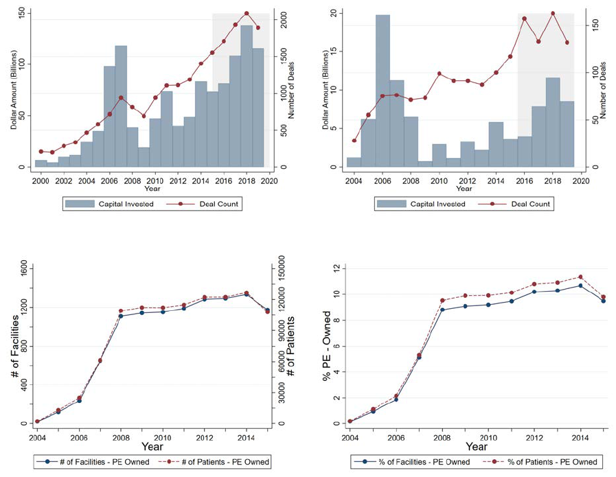
Figures and Tables
Figure 1: Private Equity Ownership in Healthcare
A: PE Deals in Healthcare B: PE Deals in Eldercare
C: Number of Facilities and Patients Acquired D: Percentage of Facilities and Patients Acquired
Note: This figure shows PE deals in health care over time. Panels A and B present the total capital invested (left
axis) and number of transactions (right axis) by PE firms in healthcare and eldercare, by year. Panels C and D
focus on the number of active nursing homes owned by PE firms in each year. Panel B presents the number of
PE-owned facilities (left axis) and patients admitted at these facilities (right axis). Note that the total number of
facilities ever bought by PE firms is larger (1,674) than what is plotted here since some of these facilities closed
or went back to non PE ownership over time. Panel D presents these trends as a percentage of total number of
facilities and patients admitted, respectively.
37
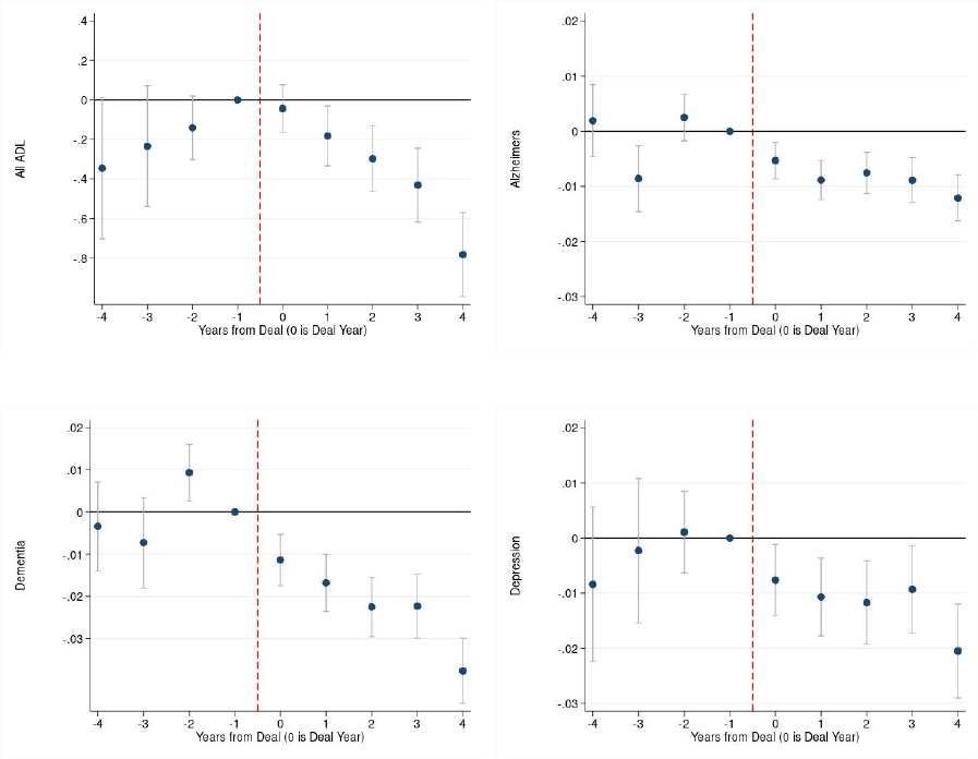
Figure 2: Initial Patient Assessments
A: ADL Score B: Alzheimers
C: Dementia D: Depression
Note: This figure presents event studies on initial patient assessments around the time a nursing home experiences
a PE buyout. We estimate these models on collapsed facility-year level data. Each point in the figures represents a
coefficient obtained by estimating an event study version of Equation (1). The model is fully saturated, including
coefficients for all years except Year = -1, which is the omitted point, but we plot only years -4 to 4. Panel
A presents results on activities of daily living (ADL) score for patients where a higher score indicates more
dependence, Panel B on an indicator for Alzheimer’s, Panel C on an indicator for Dementia, and Panel D on an
indicator for Depression, respectively, at admission to the index nursing home stay. Standard errors are clustered
by facility.
38

Figure 3: Patient Characteristics with Differential Distance
A: High Risk Patients
B: Stay at PE Nursing Home
Note: This figure presents scatter plots of patient characteristics against differential distance to the nearest PE
facility. The independent variable is the difference in distance (in miles) of the nearest PE nursing home to the
nearest non-PE nursing home for the patient. The dependent variable in Panel A is an indicator for the patient
to have a Charlson Co-morbidity Index (based on diagnoses recorded in hospital inpatient and outpatient claims
over the 3 months before admission to nursing home) greater than 2, and in Panel B is an indicator for the nursing
home being PE-owned. The data was collapsed into 10 equal sized bins and we plot the means of residuals in
each bin that were obtained from models including facility and patient HRR x Year fixed effects, and patient
demographics: age, race, gender, maritial status, and an indicator if patient is dual eligible. Panel B additionally
controls for indicators for 17 pre-existing conditions used to compute the Charlson Index. The figures also present
quadratic fitted lines for these plots. Each plot also presents the slope coefficient (per 10 miles of differential
distance) with the corresponding standard error. Standard errors are clustered by facility.
39
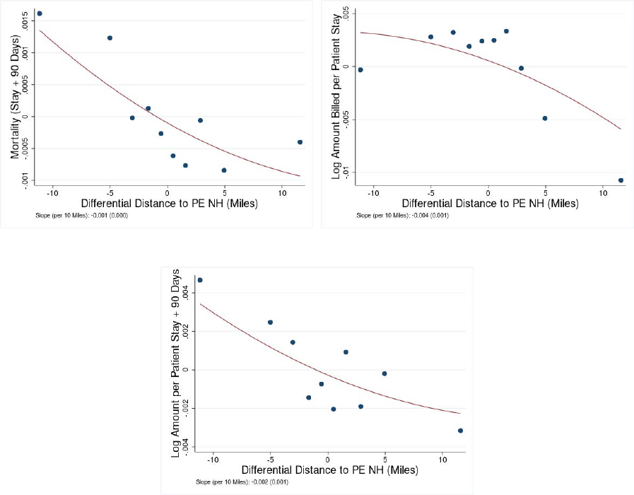
Figure 4: Patient Outcomes with Differential Distance
A: Mortality (Stay + 90 Days) B: Log Amount Billed per Patient Stay
C: Log Amount Billed per Patient Stay + 90 Days
Note: This figure presents scatter plots of patient characteristics against differential distance to the nearest PE
facility. The independent variable is the difference in distance (in miles) of the nearest PE nursing home to the
nearest non-PE nursing home for the patient. The dependent variable in Panel A is an indicator for patient death
during or 90 days post nursing home stay, in Panel B refers to log of the total payment for the index nursing
home stay, and in Panel C is the log of the total payment for index stay and 90 days post nursing home stay. The
data was collapsed into 10 equal sized bins and we plot the means of residuals in each bin that were obtained
from models including facility and patient HRR x Year fixed effects, and patient demographics: age, race, gender,
maritial status, indicators for 17 pre-existing conditions used to compute the Charlson Index, and an indicator if
patient is dual eligible. The figures also present quadratic fitted lines for these plots. Each plot also presents the
slope coefficient (per 10 miles of differential distance) with the corresponding standard error. Standard errors are
clustered by facility.
40
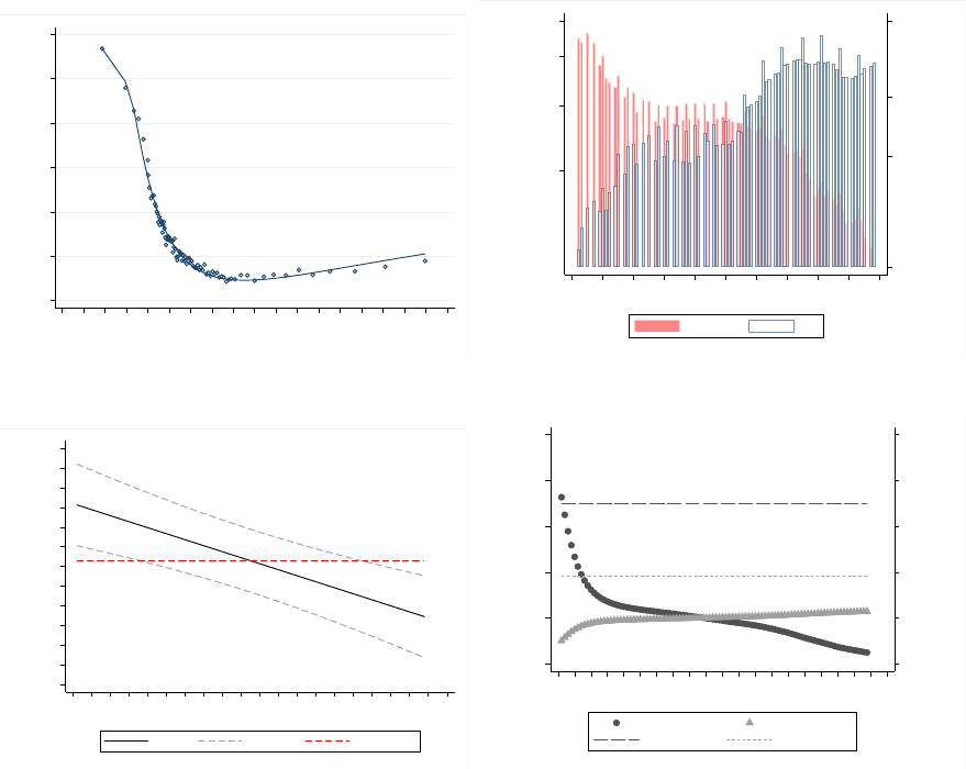
Figure 5: Marginal Treatment Effects
0.0
0.1
0.2
0.3
0.4
0.5
0.6
P(z)
-20 -10 0 10 20 30 40 50 60 70
Differential distance (miles)
A: First stage
50
1,000
5,000
40,000
Number of PE
500
10,000
100,000
500,000
Number of non-PE
0 .2 .4 .6 .8 1
Propensity Score
Non-PE PE
B: Common Support
-0.04
-0.03
-0.02
-0.01
0.00
0.01
0.02
0.03
0.04
0.05
0.06
0.07
0.08
MTE
0.0 0.1 0.2 0.3 0.4 0.5 0.6 0.7 0.8 0.9 1.0
Unobserved resistance to treatment
MTE 90% CI ATE (.023)
C: MTE curve
0.000
0.010
0.020
0.030
0.040
0.050
Treatment effect
0.000
0.010
0.020
0.030
0.040
0.050
Weights
0.0 0.1 0.2 0.3 0.4 0.5 0.6 0.7 0.8 0.9 1.0
Unobserved resistance to treatment
TT weights TUT weights
ATT (.035) ATUT (.019)
D: ATT and ATUT
Note: This figure presents results pertaining to Marginal Treatment Effects (MTE) analysis using the Medicare
patient-level data. Panel A presents the ‘first stage’ fit of predicted probability of treatment or propensity score,
w.r.t the instrument. Panel B presents the overlap in distributions of PE and non-PE groups by propensity score.
This plot uses a log scale due to the large number of non-PE patients with low propensity. Panel C presents the
weights for the IV and corresponding estimates. Panel D presents the weights for the Average Treatment on the
Treated (ATT) and Average Treatment on the Untreated (ATUT) and the corresponding estimates. Section 5.2
describes the MTE estimation.
41
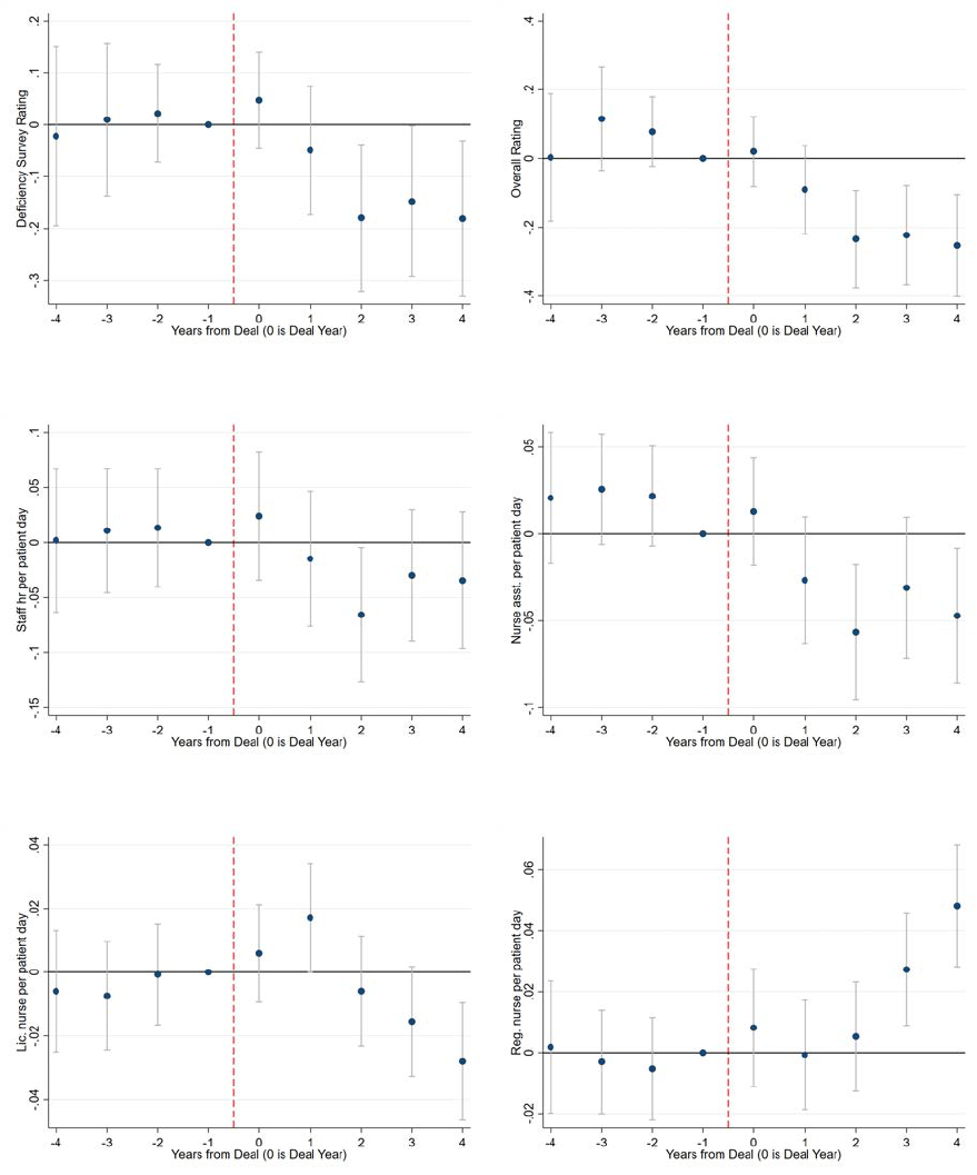
Figure 6: Aggregate Quality and Staffing Outcomes
A: Deficiency Survey Rating B: Overall Rating
C: Staff Hour per Patient Day D: Nurse Asst. per Patient Day
E: Lic. Nurse per Patient Day F: Registered Nurse per Patient Day
Note: This figure presents event studies on quality of care measures (Five Star ratings) and Staffing around the
time a nursing home experiences a PE buyout. Each point in the figures represents the coefficient β
s
obtained by
estimating Equation (5) as discussed in Section 6. The model is fully saturated, including coefficients for all years
except Year = -1, which is the omitted point, but we plot only years -4 to 4. In Panels A and B, we present effects
on the Five-star ratings awarded by CMS - deficiencies identified by independent contractors in audits and overall
rating, respectively. A negative effect on ratings implies a decline in quality. Panels C to F present results on nurse
staffing per-patient for all staff, nurse assistants, licensed nurses, and registered nurses respectively. All models
include facility and year fixed effects, patient mix and market controls, as described in Section 6.1. All dependent
variables are winsorized at 1 and 99% level. Standard errors are clustered by facility.
42
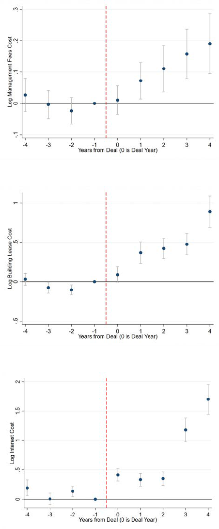
Figure 7: Facility Finances
A: Log Management Fee Cost
B: Log Building Lease Cost
C: Log Interest Cost
Note: This figure presents event studies on facility finances around the time a nursing home experiences a PE
buyout. Each point in the figures represents the coefficient β
s
obtained by estimating Equation (5) as discussed
in Section 6. The model is fully saturated, including coefficients for all years except Year = -1, which is the
omitted point, but we plot only years -4 to 4. Panels A to C present results on the log of management fee cost,
building lease cost, and interest cost, respectively. All models include facility and year fixed effects, patient mix
and market controls, as described in Section 6.1. All dependent variables are winsorized at 1% and 99% levels.
Standard errors are clustered by facility.
43

Table 1: Descriptive Statistics
All
Not PE Owned PE Owned
Mean
SD Count Mean Count Mean Count
A.
Facility Level Attributes
Overall Five-Star Rating 3.05 1.29 111,807 3.07 101,044 2.83 10,763
Deficiency Five-Star Rating 2.76 1.24 111,807 2.77 101,044 2.62 10,763
Staff Hours per Pat. Day 3.44 1.32 227,446 3.44 214,456 3.38 12,990
Nurse Assistant Hours per Pat. Day 2.21 0.73 227,446 2.22 214,456 2.06 12,990
Licensed Nurse Hours per Pat. Day 0.81 0.42 227,446 0.81 214,456 0.82 12,990
Registered Nurse Hours per Pat. Day 0.40 0.46 227,446 0.39 214,456 0.49 12,990
Number of Beds 108.00 53.41 227,446 107.74 214,456 112.34 12,990
Admissions 186.54 162.71 227,446 181.94 214,456 262.47 12,990
Ratio Black 0.12 0.18 227,446 0.12 214,456 0.12 12,990
Ratio Medicaid 0.63 0.22 227,445 0.64 214,455 0.60 12,990
Ratio Medicare 0.14 0.15 227,445 0.14 214,455 0.18 12,990
Ratio Private 0.22 0.17 227,445 0.22 214,455 0.22 12,990
Management Fees (2016$) 7,527 116,603 197,062 6,280 184,498 25,833 12,564
Building Lease (2016$) 6,404 80,743 197,085 5,211 184,521 23,919 12,564
Interest Expense (2016$) 14,663 165,595 197,103 6,079 184,539 140,733 12,564
B.
Medicare Patient Attributes
Age 81.13 8.09 4,231,460 81.18 3,641,924 80.81 589,536
Female 0.63 0.48 4,231,460 0.64 3,641,924 0.62 589,536
Black 0.09 0.29 4,231,460 0.09 3,641,924 0.09 589,536
White 0.87 0.33 4,231,460 0.87 3,641,924 0.88 589,536
Married 0.35 0.48 4,231,460 0.35 3,641,924 0.36 589,536
Charlson Score (Previous) > 2 0.27 0.45 4,231,460 0.27 3,641,924 0.29 589,536
Cardio-Vascular Disease 0.18 0.39 4,231,460 0.18 3,641,924 0.18 589,536
Injury 0.19 0.39 4,231,460 0.19 3,641,924 0.19 589,536
Other 0.63 0.48 4,231,460 0.63 3,641,924 0.63 589,536
Dual Eligible 0.17 0.37 4,231,460 0.17 3,641,924 0.15 589,536
Differential Distance (Miles) 9.77 12.47 4,231,460 11.07 3,641,924 1.75 589,536
Mortality (Stay + 90 Days) 0.19 0.39 4,231,460 0.18 3,641,924 0.19 589,536
Uses Anti-Pyschotics 0.10 0.29 4,231,460 0.10 3,641,924 0.09 589,536
Mobility Reduces 0.53 0.50 4,231,460 0.52 3,641,924 0.62 589,536
Develops Ulcers 0.09 0.28 4,231,460 0.08 3,641,924 0.09 589,536
Pain Intensity Increases 0.26 0.44 4,231,460 0.26 3,641,924 0.30 589,536
Amount Billed per Patient Stay (2016$) 13,100 11,400 4,231,460 13,000 3,641,924 13,400 589,536
Amount Billed per Patient Stay + 90 Days (2016$) 20,800 20,100 4,231,460 20,700 3,641,924 21,100 589,536
Note: This table presents descriptive statistics for key variables used in the analysis. Panel A presents descriptives
on facility-level data for all for-profit nursing homes over the years 2000–17 while Panel B presents patient-level
data for Medicare patients with index stays over the years 2005–16. A unit of observation is a facility-year in
Panel A and a unique patient in Panel B (since we retain only the first stay per patient). Columns 1, 2 and 3
present means, standard deviations and number of observations for the full sample. We categorize facilities into
two groups. Columns 4 and 5 present means and number of observations at facilities that never experienced a PE
acquisition or before PE acquisition during our sample period. Columns 6 and 7 present corresponding values
for facilities in the post-buyout period. For most variables, about 10% of the observations pertain to facilities
that experienced a PE acquisition. Sample sizes differ across variables in Panel A since they were sourced from
multiple sources or in some cases were reported only for more recent years. In Panel A, all continuously varying
variables were winsorized at the 1% and 99% levels. We compute the Charlson Co-morbidity Index using co-
morbidities diagnosed in hospital inpatient and outpatient claims (first 10 dx codes) over the 3 months prior to, but
not including, the index stay. Spending values in Panel B are winsorized at the 99% level and deflated to be in 2016
dollars. ‘Total’ billing includes hospital inpatient, outpatient including emergency department, and nursing home
stay spending over the 90 days following discharge from the index stay and includes the index stay. The following
patient-level variables were sourced from the Minimum Data Set (MDS): marriage, mobility, pressure ulcers, and
pain intensity. Medicare patients that could not be merged into the MDS (94% match rate) were dropped from the
sample. Facilities with less than 100 Medicare patients over the entire period were omitted from the patient-level
sample. If any of the MDS variables was missing, then we set the respective indicator to zero. We exclude patients
facing an absolute magnitude of differential distance of greater than 20 miles.
44

Table 2: Effect of Private Equity Buyouts on Patient Outcomes
A:
Initial Patient Assesments (OLS Estimates)
(1)
(2) (3) (4)
ADL Score Alzheimers Dementia Depression
At Admission At Admission At Admission At Admission
1(PE)
-0.1124* -0.0047*** -0.0157*** -0.0060**
(0.062) (0.001) (0.002) (0.002)
Observations 3,962,599 3,962,599 3,962,599 3,953,806
Y-Mean 15.90 0.05 0.17 0.25
B:
OLS Estimates
(1)
(2) (3)
Mortality Log Amount Billed Log Amount Billed
(Stay + 90 Days) Per Patient Stay Per Patient Stay + 90 Days
1(PE)
0.0030** -0.0258*** -0.0163***
(0.001) (0.006) (0.005)
Observations 4,231,356 4,231,356 4,231,356
Y-Mean 0.18 9.05 9.56
C:
IV Estimates
(1)
(2) (3)
Mortality Log Amount Billed Log Amount Billed
(Stay + 90 Days) Per Patient Stay Per Patient Stay + 90 Days
1(PE)
0.0195*** 0.0768*** 0.0604***
(0.007) (0.025) (0.021)
Observations 4,231,356 4,231,356 4,231,356
Y-Mean 0.18 9.05 9.56
F-Stat 243 243 243
D:
Placebo Analysis (IV Estimates)
(1)
(2) (3)
Mortality Log Amount Billed Log Amount Billed
(Stay + 90 Days) Per Patient Stay Per Patient Stay + 90 Days
1(PE)
0.002 -0.0215 -0.0241*
(0.004) (0.016) (0.013)
Observations 3,710,981 3,710,981 3,710,981
Y-Mean 0.20 9.02 9.53
F-Stat 590 590 590
Note: This table presents estimates of the relationship between PE ownership and patient health and spending. Panel
A presents OLS results for initial assessments of patients entering nursing homes, obtained by estimating Equation
(1). In Panel B, each cell presents the coefficient β obtained by estimating Equation (1). The independent variable is
an indicator for the patient being admitted to a PE nursing home. We present effects for claims-based patient quality
outcomes - patient death within 90 days of discharge from the index stay, and total amount billed (2016$). Panel C
presents the coefficient β for the same outcomes obtained by estimating Equation (3) by 2SLS, with the indicator for
the patient being admitted to a PE nursing home, instrumented by differences in distance to the nearest PE and non-PE
facility. Panel D presents these results from a placebo analysis of the relationship between private equity ownership and
patient health and spending. We assign placebo PE acquisition to three years before the actual acquisition and discard
data for any facility starting with the year it actually got acquired. Accordingly we re-compute differential distance
values taking into account these placebo acquisitions. All regressions include facility and patient HRR x Year fixed
effects, and patient risk controls. Patient risk controls include age, race, gender, marital status, indicators for 17 pre-
existing conditions used to compute the Charlson Index, and an indicator if patients are dual eligible. Standard errors
are clustered by facility. *p < .1, ** p < .05, *** p < .01.
45

Table 3: Patient-Level Analysis: First Stage
(1) (2) (3) (4)
1(PE) 1(PE) 1(PE) 1(PE)
Differential Distance -0.0699*** -0.0699*** -0.0698*** -0.0451***
(In 10 Miles) (0.003) (0.003) (0.003) (0.002)
(Differential Distance)
2
0.0092*** 0.0092*** 0.0091*** 0.0066***
(In 10 Miles) (0.001) (0.001) (0.001) (0.001)
Facility FEs Y Y Y Y
Patient Controls Y Y Y
Zipcode Controls Y
Patient FEs Level HRR x Year HRR x Year HRR x Year HSA x Year
Observations 4,231,356 4,231,356 4,227,196 4,230,487
Y-Mean 0.14 0.14 0.14 0.14
F-Stat 243 243 241 220
Note: This table presents estimates of the relationship between PE ownership of the nursing home and the patient’s
differential distance. Each cell presents the coefficient β obtained by estimating Equation (2). The independent
variable is the difference in distance (both linear and quadratic, in 10 miles) to the nearest PE nursing home and the
nearest non-PE nursing home for the patient. This is calculated based on distances between the respective zip code
centroids. The outcome variable is an indicator for whether the nursing home serving the patient is PE-owned (=1
if PE-owned, 0 otherwise). Column 1 controls for facility and patient market (Hospital Referral Region) x Year
fixed effects. Column 2 (our preferred specification) adds controls for patient risk controls (indicators for 17 pre-
existing conditions used to define the Charlson Co-morbidity Index inferred from claims over the three months
prior to admission, and sex, age, race, marital status, and an indicator if patients are dual eligible). Column 3
adds controls for patient zip-year characteristics: median household income, the shares of the population that are
white, that are renters rather than home-owners, that are below the Federal poverty line, and that are enrolled in
the medicare advantage program. Column 4 uses the same controls as in column 2 but defines patient market
using a narrower market definition: Hospital Service Area (HSA) instead of HRR. Standard errors are clustered
by facility. *p < .1, ** p < .05, *** p < .01.
46

Table 4: Balance of Patient Characteristics
(1) (2)
Patient Attribute DD < Median DD > Median
Differential Distance 1.63 17.91
PE Owned Nursing Home 0.24 0.04
Age 81.10 81.16
Female 0.63 0.64
Black 0.10 0.08
Married 0.35 0.34
Charlson Score Categories:
Dual Eligible 0.15 0.18
AMI 0.08 0.08
Congestive Heart Failure 0.23 0.24
PVD 0.06 0.05
CEVD 0.13 0.14
Dementia 0.04 0.04
COPD 0.22 0.23
Rheumatoid Arthritis 0.03 0.03
Peptic Ulcer 0.02 0.02
Mild Liver Disease 0.01 0.01
Diabetes 0.21 0.22
Diabetes + Complication 0.04 0.04
Paraplegia 0.03 0.03
Renal Disease 0.14 0.13
Cancer 0.09 0.09
Severe Liver Disease 0.01 0.01
Metastatic Cancer 0.04 0.04
AIDS 0.00 0.00
Initial Assessments:
ADL Score At Admission 15.89 15.87
Alzhiemers At Admission 0.05 0.06
Dementia at At Admission 0.17 0.17
Depression at Admission 0.25 0.26
Number Of Patients 2,116,500 2,114,960
Note: This table presents the balance in patient attributes with respect to the
instrument: differential distance. We divide patients into two groups based on whether
their differential distance is below or above the median value (8.9 miles). Recall
that differential distance (DD) is the difference between distance to the nearest PE
nursing home and the nearest non-PE nursing home for the patient. Column 1 presents
the means of patient characteristics for patients with DD below the median value,
while Column 2 presents the means for patients with DD greater than the median.
We present patient demographics, 17 co-morbidity indicators used to compute the
Charlson Co-morbidity Index, and 4 initial assessment characteristics of patients at
the time of admission to the index nursing home stay from the Minimum Data Set.
Charlson score categories were coded using diagnosis codes on hospital inpatient and
outpatient claims over the 3 months prior to, but not including, the index nursing
home stay. Paraplegia includes both partial and complete paralysis. We generated
indicators for the Charlson score disease categories using the ‘charlson’ command in
Stata, available at http://fmwww.bc.edu/RePEc/bocode/c/charlson.html.
47

Table 5: Patient-Level Analysis: Robustness
(1)
(2) (3)
Mortality Log Amount Billed Log Amount Billed
(Stay + 90 Days) Per Patient Stay Per Patient Stay + 90 Days
1.
Base Specification
1(PE) 0.0195*** 0.0768*** 0.0604***
(0.007) (0.025) (0.021)
2. Varying Controls
A. No Controls
1(PE) 0.0285*** 0.1162*** 0.0634***
(0.008) (0.026) (0.022)
B. Zip-Year Controls
1(PE) 0.0187*** 0.0776*** 0.0599***
(0.007) (0.025) (0.021)
C. HSA-Year FEs
1(PE) 0.0402*** 0.1113*** 0.1286***
(0.015) (0.043) (0.038)
3. Changed distance threshold
A. Narrower Distance Threshold
1(PE) 0.0177** 0.0508** 0.0406*
(0.007) (0.025) (0.021)
B. Wider Distance Threshold
1(PE) 0.0181** 0.0986*** 0.0729***
(0.007) (0.025) (0.021)
4. Alternate functional form
1(PE) 0.0297*** 0.1423*** 0.1060***
(0.010) (0.032) (0.028)
5. Clustering by Deals
1(PE) 0.0195** 0.0769*** 0.0604**
(0.009) (0.028) (0.028)
6. Corporatization
A. Include Chain Controls
1(PE) 0.0195*** 0.0769*** 0.0604***
(0.007) (0.025) (0.021)
B. Top 5 Deals Only
1(PE) 0.0408*** 0.1017** 0.0866**
(0.012) (0.040) (0.035)
7. Excluding select deals
A. W/O Top 2 Deals
1(PE) 0.0330*** 0.1034*** 0.0929***
(0.011) (0.038) (0.032)
B. Excluding Formation and Fillmore Capital
1(PE) 0.0426*** 0.1088** 0.1300***
(0.013) (0.044) (0.038)
8. Excluding Top 5 States with Retirement Inflows and Outflows
1(PE) 0.0188** 0.0891*** 0.0739***
(0.008) (0.027) (0.023)
Observations 4,231,356 4,231,356 4,231,356
Y-Mean 0.18 9.05 9.56
Note: This table presents results from specification checks on the relationship between PE ownership and patient health and
spending, corresponding to results in Panel A in Table 2. The first panel presents the base specification. The second panel
presents results by varying controls: row 2A presents coefficients from a model with fixed effects only, row 2B includes
patient zip controls: median household income, the shares of the population that are white, that are renters rather than home-
owners, that are below the federal poverty level, and that are enrolled in Medicare Advantage program, and while all other
rows include HRR x year fixed effects, and row 2C uses Hospital Service Areas (HSA) instead of HRR. The third panel
tests robustness to varying the distance threshold to include patients. Rows 3A and 3B exclude all patients whose zipcode
has a minimum differential distance of more than 15 miles and 25 miles, respectively. The fourth panel uses an indicator of
differential distance greater than median value rather than actual differential distance for the estimates. The fifth panel clusters
estimates by deals instead of facilities. The sixth panel checks if results are driven by PE ownership or corporatization: row
6A controls for facility being part of a chain, and row 6B limits the PE group to only the facilities bought in the 5 largest PE
deals. The seventh panel presents various sample cuts: row 7A calculates the results excluding all data for chains involved
in the 2 largest PE deals, and row 7B excludes all deals with Formation and Fillmore Capital. The eighth panel excludes
five states with largest retiree inflows and outflows. All rows (except 2A) include patient risk controls: age, race, gender,
marital status, indicators for 17 pre-existing conditions used to compute the Charlson score, and an indicator if patients are
dual eligible. Standard errors are clustered by facility (except for fifth panel). *p < .1, ** p < .05, *** p < .01.
48

Table 6: Heterogeneity in Patient Mortality
(1) (2) (3) (4)
Observations Mean Coefficient (Std. Errors)
A: Patient Level Characteristics
1. Risk
Low Risk 3,073,198 0.14 0.0197** (0.008)
High Risk 1,157,836 0.29 0.0216 (0.014)
2. Gender
Male 1,547,356 0.23 0.0202* (0.012)
Female 2,683,713 0.16 0.0186** (0.008)
3. Length of Stay
Length of Stay < Median 2,159,020 0.22 0.0342*** (0.011)
Length of Stay > Median 2,072,060 0.15 0.0094 (0.009)
4. Discharge Location
Home 2,420,039 0.06 0.0070 (0.006)
Facility 1,098,419 0.35 0.0826*** (0.018)
Other 712,213 0.34 0.0042 (0.016)
5. Health Diagnosis for Discharge to Facility
Injury and Infection 210,194 0.47 0.1194*** (0.043)
Cardio-Vascular 297,548 0.45 0.0399 (0.033)
Other 320,423 0.41 0.0582* (0.031)
B: Facility Level Characteristics
1. Urban Indicator
Rural 870,421 0.20 0.0139 (0.012)
Urban 3,360,790 0.18 0.0260*** (0.010)
2. Log(Beds)
Log(Beds) < Median 1,322,962 0.17 0.0324** (0.013)
Log(Beds) >= Median 2,908,277 0.19 0.0134 (0.009)
3. Admits per Bed
Admits Per Bed < Median 604,084 0.23 0.0323 (0.022)
Admits Per Bed >= Median 3,627,022 0.18 0.0156** (0.008)
Note: This table presents heterogeneity in the effects of PE ownership on patient mortality. Column 1
presents the sample size and Column 2 presents the corresponding mean mortality. Columns 3 and 4
present the corresponding coefficient β and its standard error obtained by estimating Equation (3) by
2SLS. The independent variable is the indicator for a patient being admitted to a PE nursing home,
instrumented by differences in distance to the nearest non-PE and PE nursing home. The outcome
variable is an indicator for patient death within 90 days of discharge from the index stay. Panel A
explores the heterogeneity on several patient level factors - by dividing patients into 2 groups based on
severity of pre-existing co-morbidities (high risk = Charlson Index greater than 2) in row 1, gender in
row 2, length of stay (above and below median) in row 3, patient discharge location in row 4, and the
reason for discharge to facility in row 5. Panel B explores the heterogeneity on several facility level
factors - by dividing facilities based on facilities being in Urban counties in row 1, facility size in row
2, facility admits per bed in row 3. All models include facility and patient HRR x year fixed effects.
We additionally control for the usual patient risk controls as in the main regression. Standard errors
are clustered by facility. *p < .1, ** p < .05, *** p < .01.
49

Table 7: Patient Wellbeing
A: OLS Estimates
(1) (2) (3)
1(Mobility 1(Develops 1(Pain Intensity
Decreases) Ulcers) Increases)
1(PE) 0.0321*** 0.0068** 0.0272***
(0.003) (0.003) (0.005)
Observations 4,231,356 4,231,356 4,231,356
Y-Mean 0.52 0.08 0.26
B: IV Estimates
(1) (2) (3)
1(Mobility 1(Develops 1(Pain Intensity
Decreases) Ulcers) Increases)
1(PE) 0.0152* -0.005 0.0216
(0.009) (0.007) (0.014)
Observations 4,231,356 4,231,356 4,231,356
Y-Mean 0.52 0.08 0.26
Note: This table presents estimates of the relationship between PE ownership and measures of patient wellbeing
obtained from clinical assessments. Each cell in Panel A presents the β obtained by estimating Equation (1),
and each cell in Panel B presents the IV version of the same results, obtained by estimating Equation (3). The
independent variable is an indicator for the patient being admitted to a PE nursing home in Panel A, and is
instrumented by differences in distance to the nearest PE and non-PE facility in Panel B. We present results for
patient level outcomes - an indicator for decrease in patient mobility, developing/worsening pressure ulcers, and
increase in pain intensity. All models include facility and patient HRR x Year fixed effects. We additionally control
for the usual patient risk controls as in the main regression. Standard errors are clustered by facility. *p < .1, **
p < .05, *** p < .01.
50

Table 8: Mechanisms and Operational Changes
A: Five Star Rating
(1) (2)
Deficiency Overall
Rating Rating
1(PE) -0.077** -0.083**
(No Control) (0.037) (0.036)
1(PE) -0.080** -0.086**
(With Control) (0.037) (0.036)
Observations 111,728 111,728
Y-Mean 2.8 3.1
B: Staff Per Patient Day
(1) (2) (3) (4)
All Staff Nurse Assistant Licensed Nurse Registered Nurse
1(PE) -0.046*** -0.062*** -0.024*** 0.039***
(No Control) (0.017) (0.010) (0.006) (0.005)
1(PE) -0.042** -0.060*** -0.023*** 0.040***
(With Control) (0.017) (0.010) (0.006) (0.005)
Observations 227,254 227,254 227,254 227,254
Y-Mean 3.4 2.2 0.8 0.4
C: Log Financials
(1) (2) (3)
Management Fee Building Lease Interest Expense
1(PE) 0.056* 0.570*** 1.179***
(No Control) (0.032) (0.061) (0.096)
1(PE) 0.056* 0.570*** 1.174***
(With Control) (0.032) (0.061) (0.096)
Observations 196,880 196,900 196,918
Y-Mean 0.2 0.4 0.3
Note: This table presents estimates of the relationship between PE ownership and nursing home outcomes. Each
cell presents the coefficient β obtained by estimating equation 4 with a different outcome. The independent variable
is an indicator for whether a nursing home is PE-owned (=1 if PE-owned, 0 otherwise) starting in the next year
from the deal announcement date. Panel A presents results for quality outcomes as measured by Five-star rating
awarded by CMS - overall rating and deficiencies identified by independent contractors in audits, respectively. A
negative effect on ratings implies a decline in quality. Panel B presents results on per patient nurse availability
for all nurses, nurse assistants, licensed nurses, and registered nurses. Panel C presents results on the log of
management fees, building lease cost, and interest expenses. The top row presents results with no controls. The
bottom row presents the results including controls, which consist of market-level and patient mix controls, as
described in Section 6.1. All models include facility and year fixed effects. All variables are winsorized at 1% and
99% levels. Standard errors are clustered by facility. *p < .1, ** p < .05, *** p < .01.
51

Appendix: For Online Publication
A Data appendix
This paper uses three primary data sources. We use (1) publicly available nursing home-level
data, (2) patient-level administrative claims data, both obtained from CMS, and (3) Pitchbook
data on PE deals. This section provides a detailed explanation of these data sources and how
we arrived at our analysis samples.
A.1 Nursing Home Data
Our data source on nursing home-level operations and performance is a compilation of
information obtained during annual surprise CMS inspector audits and data on nursing home
attributes and patient characteristics reported by the facilities themselves.
39
The data span
2000 through 2017. In each year we observe about 15,000 unique nursing homes, for a total of
approximately 280,000 observations. Of these, about 13,000 observations represent facilities
acquired by PE firms. The aggregate files provide annual data on basic facility attributes,
patient volume and case mix, nurse availability, and various components of the Five Star
ratings.
40
These ratings started in 2009, so we cannot observe ratings pre-buyout for deals
before 2010. Fortunately, half of the PE deals in our sample, accounting for 365 nursing
homes, occurred post-2009.
Table 1 Panel A presents summary statistics on the Overall Five Star rating as well as
the other key nursing home-level variables used in the analysis. We first present the mean
and standard deviation for the whole sample (columns 1-2), then divide observations into two
groups—for facilities that are not PE-owned (columns 4-5) and for those that are (columns 6-7).
We observe clear differences between PE-owned facilities and those not owned (all statistically
significant at the 1% level except where noted). PE targets are slightly larger, have fewer staff
hours per resident, and a lower Overall Five Star rating. There have been secular increases for
the whole sector in both ratings and staffing over time. For staffing, this reflects more stringent
standards from regulators over time. Average staff hours per patient day increased from 3.5 in
2000 to 3.7 in 2017. Similarly, overall average Five Star ratings increased from 2.9 in 2009 to
3.25 in 2017. As the PE deals occurred primarily later in the sample, it is therefore remarkable
that they have lower measures of quality on average.
A.2 Patient Data
Our second data source consists of patient-level billing claims and assessment data for
Medicare fee-for-service beneficiaries from 2005 to 2016. We observe the universe of billing
data for hospital care (inpatient and outpatient) and nursing homes for these beneficiaries, as
well as detailed patient assessments recorded in the Minimum Data Set (MDS).
41
We use
these files to track beneficiaries’ demographics, spending, and health outcomes such as
mortality. The MDS helps observe clinical assessments such as mobility.
39
These files were organized and made available for research by the Long Term Care Focus research center at
Brown University. See www.ltcfocus.org for more details.
40
For more details on how the ratings are produced, see Rating Guide.
41
Specifically, we use 100% samples of the following: Medicare Beneficiary Summary File (MBSF), Hospital
inpatient and outpatient, and Skilled Nursing Facility claims files. These were obtained through a reuse DUA with
CMS and accessed through the NBER.
52

The unit of observation is a nursing home stay for a Medicare beneficiary that begins during
our sample period, which we begin in 2005 in order to have at least one look-back year. Our
main sample restriction is to identify index nursing home stays for patients, defined as stays
that begin at least a year after discharge from a previous nursing home stay. This helps avoid
mis-attributing adverse effects to the wrong nursing home. To further avoid attribution error,
we consider only the patient’s first index stay in our entire sample period. Hence, each patient
appears only once in our sample. Using this approach, we settle on a sample of more than 5.3
million patients over 12 years. For each of these patients, we also observe clinical assessments
from the MDS, which we successfully match to the claims files. Following the prior literature
(Grabowski et al., 2013), we use some other restrictions to arrive at our sample. We restrict to
patients over 65 years of age who are enrolled in Medicare parts A and B for at least 12 months
before the start of the nursing home stay. This restriction ensures that we observe prior medical
care history and pre-existing conditions. We also restrict to stays associated with a hospital
visit in the previous month, so that all patients are admitted after a hospital-based procedure
and are relatively homogeneous. We drop patients who went to a nursing home in a state other
than their state of residence as recorded in the Medicare master beneficiary summary file. This
drops a small fraction of patients (less than 5%) and is meant to exclude patients who may
be traveling when admitted to a nursing home. Following convention, we drop patients facing
a large differential distance value. We exclude zip codes based on the absolute magnitude of
the differential distance, treating patients very close to PE facilities the same as those very far
away. In practice very few zip codes are more than 20 miles closer to a PE facility. Differential
distance values update for some zip codes over time as facilities are acquired or sold by PE
firms. We exclude such zip codes only if their differential distance remains more than 20 miles
in magnitude throughout. We match the index nursing home stays to the MDS sample on
beneficiary ID, facility ID, and admission date. We achieve a match rate of 94% and drop
unmatched patients. We drop facilities with fewer than 100 patients over the entire sample
period to avoid special facilities and mitigate noise.
Table 1 Panel B presents summary statistics on the final patient-level sample. We use an
indicator for death within 90 days following discharge (including during the stay), based on
death dates recorded in the Medicare master beneficiary summary file. We use two measures of
spending. The first is the total amount that the nursing home bills to Medicare and the patient
for the index stay in 2016 dollars. Medicare covers the entire cost until the 21st day of stay, at
which point the patient begins paying a coinsurance, which has risen somewhat over time and
is now $170.5 per day.
42
In our data, about 90% of total payments are by Medicare. PE-owned
facilities charge about 10% more than other facilities. The second measure is the total amount
paid for the stay and the 90 days following discharge. This captures any subsequent hospital
inpatient or outpatient care, and it provides a more holistic picture of patient care.
Demographic measures associated with risk are quite similar across the types of facilities,
including patient age, the share of patients who are black and married, and the Charlson
Comorbidity Index, a standard measure of patient mortality risk based on co-morbidities
(Charlson et al., 1994).
43
We create a high-risk indicator that is one if the previous-quarter
Charlson score is greater than two. According to this definition, about 30% of patients are
high-risk. The difference between facility types is not significant.
Finally, we examine three measures of patient well-being which comprise inputs to the
42
See https://www.resdac.org/cms-data/files/ip-ffs/data-documentationandhttps:
//www.medicare.gov/Pubs/pdf/10153-Medicare-Skilled-Nursing-Facility-Care.pdf.
43
The “Charlson score" assigns a point score to each of 17 disease categories recorded during the 3 months
before the index stay and sums them to create an overall disease burden score.
53

quality portion of CMS’ Five Star ratings. The first is an indicator for the patient’s self-reported
mobility score declining during the stay. The second is an indicator for developing a pressure
ulcer. The third is an indicator for the patient’s self-reported pain intensity score increasing
during the stay.
A.3 PE Deal Data
Our primary source of data on PE transactions is a proprietary list of deals in the “Elder and
disabled care” sector compiled by Pitchbook Inc., a leading market intelligence firm in this
space. The deals span 2004 to 2015. We match the target names to individual nursing facilities
using name (facility or corporate owner) and address as recorded in CMS data.
44
Target names
in these deals typically refer to holding companies, which often do not reflect the names of
individual facilities. The matching process required manual Internet searches to confirm chain
affiliations. We supplement the Pitchbook data in two ways. First, we conduct additional
Internet searches that yielded a small number of PE deals not reported by Pitchbook. Second,
we obtain a list of merger and acquisition deals from 2005 to 2016 from Levin Associates, a
market intelligence firm that tracks the healthcare sector. This helps us to identify facilities that
did not experience a new PE deal, but were acquired by an existing PE-owned chain.
45
This process yielded 128 deals, which correspond to a change in ownership to PE for 1,674
facilities. The deals are spread over time (no particular year or part of the business cycle
dominates) and across PE firms. Figure C.1 shows the number of deals in each year. In total,
our data contain 90 unique PE firms that acquired nursing homes. Most deals are syndicated and
involve multiple PE firms. Table C.1 presents the top 5 deals by number of facilities acquired.
Deal sizes are skewed, with the top 5 deals accounting more than half the facilities acquired.
On average, we observe PE-owned facilities for eight years post-acquisition.
46
It is difficult to ascertain whether we comprehensively capture PE activity in this sector.
While there is no ‘official’ tally of PE-owned nursing homes to benchmark against, our sample
size compares favorably against an estimate of 1,876 nursing homes reportedly acquired by
PE firms over a similar duration, 1998–2008 (GAO, 2010). Nonetheless, our analysis likely
underestimates the extent of PE activity in nursing homes, as matching between Pitchbook
deals and individual facilities is very challenging.
To understand whether deals are concentrated in particular regions, we plot the location of
PE-owned facilities across the U.S. in Figure C.3. PE firms appear to be more active in large
metropolitan markets, and in certain states such as Florida, Texas, New York, Pennsylvania
and Massachusetts. However, there is no obvious concentration, and we do not find systematic
variation with local measures of income, age, elder population, or share of patients eligible for
Medicare Advantage.
44
We obtain data on nursing home attributes (name, address, city, owner name and type, number of beds)
and quality measures (deficiencies) from Nursing Home Compare. See https://data.medicare.gov/data/
nursing-home-compare for more details.
45
We matched approximately 290 additional facilities using information from the Levin files to the CMS data.
Of these, about 40 were PE-owned.
46
A likely source of measurement error is not capturing PE disinvestment from facility ownership. For the top
10 deals we verified PE exit via manual internet searches and incorporated it in the analysis. The main results are
robust to dropping observations of facilities that have been owned by PEs for 10 years or more. As expected, the
coefficients modestly increase in magnitude when we do so.
54

A.4 Targeting
This paper does not address why nursing homes may or may not be profitable acquisition
targets, and does not assess returns from investing. However, exploring what types of facilities
are targeted can help to interpret the effects of buyouts on patient welfare and is also useful for
identifying the most relevant control variables for our empirical analysis. We describe which
characteristics are robustly associated with buyouts in Table A.1, which presents estimates of
Equation (6):
PE
j,t
= α
s
+ α
t
+ X
0
j,t
β +
j,t
(6)
Here, PE
j,t
is set to 100 if the facility j is acquired in a PE deal in year t (we drop all years
post-deal, and multiply by 100 for ease of reading). PE
j,t
is zero for never-PE and PE-owned
facilities before the deal. We include state and year fixed effects.
We report models including variables known to be central to nursing home quality of care
and economics or that are potentially important and robustly predict buyouts. In column 1, we
find that facilities in more urban counties are more likely to be targeted.
47
Urban nursing homes
tend to be closer to hospitals and likely enjoy thicker labor markets. Facilities in a state with
a higher ratio of elderly people are also more likely to be targeted. County-level income, race,
and home ownership do not predict buyouts. Results for these covariates are not presented.
In column 2, we turn to facility characteristics. Chains are more likely to be acquired than
independent facilities, likely reflecting substantial fixed costs in deal-making. Hospital-owned
facilities are less likely to be targeted. PE firms also tend to target larger and higher-occupancy
facilities. We consider patient-level characteristics in column 3: the share of the nursing home’s
patients covered by Medicaid, the share on private insurance, and the share who are Black.
The first two are strongly negatively associated with buyouts, meaning that a higher share of
Medicare patients (the omitted group) is positively associated with being targeted. In column
4, we assess two facility-level quality measures we employ in the analysis: Five Star overall
rating and staff hours per patient day. Both are negatively associated with buyouts, but once we
control for rating, staffing is not significant. These results indicate that PE firms target relatively
low-performing nursing homes.
Finally, in column 5 we include simultaneously all of the variables from the previous models
that had predictive power. Some, such as admits per bed and hospital ownership, become small
and insignificant after controlling for the other variables. Notably, the state elder ratio, chain
indicator, and Five Star rating retain their magnitudes and precision.
47
We define urban as being in the top 2 out of 9 county groups classified as urban based on a Department of
Housing and Urban Development 2003 rural-urban classification.
55

Table A.1: Targeting
Mean (1) (2) (3) (4) (5)
Urban Indicator 0.58 0.215*** 0.140***
(0.046) (0.052)
State Elder Ratio 0.24 4.950*** 24.902***
(1.906) (5.094)
1(Chain) 0.58 0.902*** 0.413***
(0.040) (0.035)
Hospital-Owned 0.03 -0.001 0.314*
(0.134) (0.180)
Log(Beds) 4.56 0.339*** 0.091**
(0.042) (0.045)
Admits Per Bed 1.84 0.114*** 0.03
(0.015) (0.028)
Ratio Medicaid 0.64 -2.040*** -0.441
(0.213) (0.350)
Ratio Private 0.23 -2.262*** -0.262
(0.260) (0.359)
Ratio Black 0.12 -0.065
(0.116)
Overall Rating 3.02 -0.069*** -0.066***
(0.019) (0.019)
Staff Hr per Patient Day 3.41 0.017
(0.031)
Observations 184,554 171,417 171,417 81,790 81,790
Y-Mean 0.7 0.7 0.7 0.7 0.7
Note: This table shows estimates of the relationship between pre-existing nursing home characteristics and
whether a nursing home is a target of a PE buyout. Column 1 presents market-level attributes: an indicator
for urban and the share of state population which is elderly. Column 2 presents facility-level attributes: indicator
for being member of a chain, indicator for the nursing home being hospital-based, the log number of beds, and
admits per bed. Column 3 presents patient mix controls: share of patients covered by Medicaid, share of patients
who pay privately, and the share of patients who are black. Column 4 presents quality metrics such as Five-star
ratings awarded by CMS and staff hours per patient day. We re-run the regression on all variables which appear
significant in Columns 1 to 4 in Column 5. The dependent variable is 100 if the nursing home was acquired by PE
in that year and 0 otherwise. We remove all observations of private equity-owned facilities in years following the
take-over by PE. We control for state and year FEs. Standard errors are clustered by facility. *p < .1, ** p < .05,
*** p < .01.
56

B Instrument validity, robustness, and MTE details
B.1 Instrument Validation
This section discusses tests of the identification assumptions behind the instrument not
described in the main text. Two tests are related to the conditional randomization assumption.
First, PE firms may strategically target more lucrative zip codes within an HRR. If patients in
these zip codes have higher mortality, the exclusion restriction might be violated. A first test
of this possibility is to impose a more granular market definition, the Hospital Service Areas
(HSA). There are nearly 3,400 HSAs, while there are only about 300 HRRs. If neighborhood
targeting explains our result, we expect the instrument to work less well at this level. Table 3
column 4 presents results using this market definition and finds similar patterns (below, we
also show similar results in the second stage analysis). Two other tests of this hypothesis are
presented below after the main results.
Second, PE funds may strategically target nursing homes located in places with certain
desired demographic and risk profiles. We account for stable differences in the patient
catchment of facilities by including facility fixed effects. However, it is possible that PE firms
strategically target neighborhoods with desirable trends, for example with increasing
household income. We show that the results are robust to including time-varying zip
code-level socioeconomic controls. We document that these controls do not affect the first
stage in Column 3 of Table 3. We flexibly allow HRRs to evolve on different trends to mitigate
the possibility of differences in market structure confounding our results.
The monotonicity assumption implies that the first stage should be negative when
estimated on sub-samples of patients with different characteristics. Table C.2 shows that when
we estimate the relationship between below-median differential distance and PE ownership (a
simplified first stage), we recover coefficients that are very similar to the full-sample result and
all are significant at the .01 level for a variety of sample splits by age, gender, race, and
zipcode income level.
In another falsification check, following the tests proposed in Angrist et al. (2010) and
Grennan et al. (2021), we limit the sample to patient groups where we would expect
differential distance to have weak influence over facility choice. For example, patients that are
relatively very far or very close to PE facilities are likely insensitive to small changes in
distance. Similarly, patients who face similar distances to both types of facilities (within one
mile) are unlikely to choose based on this differential. Table C.4 presents results from first
stage and reduced form models (with mortality as the outcome) for such patient groups and
compares them to the main analysis sample (in column 1). The first stage is orders of
magnitude weaker for these groups, and the test statistic of joint significance for the
differential distance and its squared term is typically well below the conventional threshold for
weak instruments. These patterns reassure us that the instrument behaves according to
expectations. More importantly, we find a similar pattern for the reduced form model
coefficients. Hence, the instrument does not provide explanatory power for patient mortality in
the cases where it does not predict facility choice. This evidence counters the possibility of a
spurious relationship between differential distance and mortality.
Table C.2 also helps characterize compliers relative to the average patient at a PE facility.
The ratio of the first stage coefficient for a subsample with a specific attribute to that obtained
for the full sample provides the likelihood of compliers having that particular attribute relative
to the average PE patient.
48
Compliers appear to have a very similar age distribution (not
48
This follows from Bayes rule and the use of a discrete instrument in this model of the first stage. The
57

presented) and the probability of being male, married, or white. Intuitively, distance-based
compliers are slightly more likely to be from a low-income zipcode.
B.2 Robustness Tests
We present results from specification and falsification checks to address potential concerns
with our empirical analysis. First, we implement a placebo analysis to probe whether spurious
factors or pre-existing trends rather than the ownership change might explain the results. We use
Medicare patient-level data from 2002–07, a period with little PE ownership of nursing homes
and little overlap with our main sample (2005-16). We assign placebo PE acquisition in 2004 to
facilities that were eventually acquired before 2008 and 2005 to facilities acquired in and post
2008 by PE firms. Further, we discard data for any facility starting with the year it actually got
acquired. We recompute differential distances under these ‘placebo’ assignments and estimate
our main IV models. Table 2 Panel D presents these placebo estimates and reassuringly finds
small and insignificant effects, implying a lack of differential trends prior to acquisition.
Table 5 row 2 reports specification checks that vary the controls and market definition. If
the instrument does not randomly assign patient risk, we expect patient controls to substantially
affect the results. In row 2.A, we omit all patient controls. In row 2.B., we include zip-year
socioeconomic controls. In row 2.C, we use more granular HSAs instead of HRRs to define
patient markets. In row 3, we limit the patient sample using differential distance thresholds
of 15 miles and 25 miles instead of 20 miles. This ensures the patient sample is even more
homogeneous. In row 4, we change the functional form of our specification and use an indicator
of differential distance greater than median rather than a continuously varying value. Across
all these changes, the coefficients remain within two standard errors of the main estimates in
row 1. In row 5, we cluster standard errors by deal rather than by facility. Accordingly, the
confidence intervals widen, but the coefficients remain statistically significant.
In addition to varying the sample and right-hand side variables, we also establish that the
effect on mortality is robust to alternative durations. The results using time horizons from 15 to
365 days following discharge from the nursing home stay are shown in Table C.5. The effect
on mortality is significant and similar as a percent of the mean to the main result in all models.
For example, the effect is 10% when mortality is measured at 15 days following discharge, and
10% when measured at 365 days.
B.3 MTE estimation
This section describes the MTE model and estimation in detail, following the approach in
Cornelissen et al. (2018). We denote Y
0,i
and Y
1,i
as potential outcomes for individual i in the
untreated (k = 0) and treated (k = 1) states, respectively. Treatment in our setting is receiving
care at a PE-owned facility, PE
i
. We model these potential outcomes, Y
k,i
, as a function of
observed control vector X
i
and dummies for facility, F
j
and market-year interactions, R
r,t
. U
k,i
denotes all unobserved factors.
49
Y
k,i
= X
0
i
β
k
+ F
j
+ R
r,t
+ U
k,i
, k = 0, 1 (7)
coefficient from a subsample with attribute X is P(M|X) = P(X|M)P(M)/P(X) where M denotes a marginal PE
patient. Dividing by the first stage coefficient for the full sample, P(M), gives us P(X|M)/P(X), the relative
likelihood.
49
Following Brinch et al. (2017), we assume that the error term U
k,i
is normalized to be conditional mean zero,
i.e., E[U|X = x, F = f, R = r] = 0.
58
We then propose a latent selection model of how patients choose a PE-owned facility based on
observed and unobserved factors:
PE
∗
i
= Z
0
i
δ − V
i
,
PE
i
= 1 i f PE
∗
i
≥ 0, PE
i
= 0 otherwise,
(8)
where Z = (X, F, R, D, D
2
) is a vector including all the controls listed above in Equation (7)
and the differential distance instruments excluded from the outcome equation, D
i
and D
2
i
. We
interpret V
i
as the unobserved resistance to going to a PE-owned facility. This selection model
imposes monotonicity by using a constant parameter δ for all individuals. Following the MTE
literature, we transform the selection equation into the quantiles of the distribution of V rather
than its absolute values:
Z
0
i
δ − V
i
≥ 0 =⇒ Z
0
i
δ ≥ V
i
=⇒ Φ(Z
0
i
δ) ≥ Φ(V
i
), (9)
where Φ is the cumulative distribution function of V
i
. We interpret Φ(Z
0
i
δ) as the propensity
score, the probability that an individual with observed characteristics Z
i
chooses a PE nursing
home, and denote it as P(Z). Φ(V
i
) represents the quantiles of unobserved resistance to
treatment, and is denoted as U
D
.
Omitting subscripts for simplicity, define MT E(X = x, U
D
= u) = E[Y
1
− Y
0
|X = x, U
D
=
u]. The MTE is the treatment gain for an individual with characteristics X = x, who is in
the u
th
quantile of the resistance distribution. Such individuals are indifferent to receiving
treatment when their propensity score P(Z) = p = u. Intuitively, individuals who go to a PE
facility despite having a low value of p are revealed to have a lower resistance to treatment,
and vice-versa. Estimating the MTE for all types of patients, not just those complying with the
instrument, requires two additional functional form assumptions.
First, we assume that the MTE is additively separable into observed and unobserved
components. The observed component varies linearly with the covariates (X, F, and R), and
therefore varies by market, year, facility, and patient risk. The unobserved component depends
only on the propensity of treatment, p, which is obtained by estimating Equation 8, primarily
using the variation in differential distance. Hence, this assumption restricts the unobserved
treatment effect to be identical for all individuals at the same relative distance to a PE facility.
More technically, it eases the identification burden since we need variation in p across all
values of the covariates, rather than conditional on covariates. This assumption also implies
that treatment effect heterogeneity from X affects the MTE curve in U
D
only through the
intercept, so the slope of the MTE curve in U
D
does not depend on X.
MT E(X = x, U
D
= p) = E[Y
1
− Y
0
|X = x, U
D
= p]
= x(β
1
− β
0
)
| {z }
observed
+ E[U
1
− U
0
|U
D
= p]
| {z }
unobserved
.
. (10)
Second, we assume the unobserved component of the MTE can be approximated as a
polynomial in p. This is implemented by assuming the following outcome equation (Carneiro
et al., 2011).
E[Y|X, F, R, P(Z) = p] = X
0
β
0
+ F + R + X
0
(β
1
− β
0
)p + K(p), (11)
where K(p) is a nonlinear function of the propensity score. The derivative of this outcome
equation with respect to p estimates the marginal treatment effect at X = x and U
D
= p.
Using a polynomial aids in identification because it enables interpolation between values of p.
59
Intuitively, if mortality varies non-linearly with treatment propensity (p), the derivative w.r.t. p
would not be constant, consistent with the presence of sorting on treatment gains. If the MTE
curve slopes down in p, it implies reverse sorting, since patients who go to a PE facility despite
lower propensity and therefore exhibit lower resistance to treatment suffer a greater increase in
mortality. Figure 4A shows that mortality reduces in a concave fashion as differential distance
increases, implying mortality varies non-linearly with treatment propensity and the presence of
sorting.
We estimate the selection model in Equation (8) using a linear probability model and obtain
ˆp = Z
0
ˆ
δ. We then estimate the outcome Equation (12) below.
Y = X
0
β
0
+ F + R + X
0
(β
1
− β
0
) ˆp +
S
X
s=2
ρ
s
K( ˆp) + . (12)
The MTE curve is the derivative of Equation (12) with respect to ˆp. In our baseline model
we set S = 2 so that the MTE curve is linear in p, but we find very similar patterns using higher
order polynomials. Standard errors are obtained by block bootstrap, clustering by facility.
60
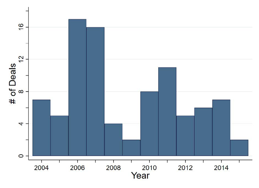
C Supplementary Figures and Tables
Figure C.1: PE Deals for Nursing Homes by Year
Note: This figure presents the number of unique deals for active nursing homes by PE firms for each year over the
period 2004–2015.
61
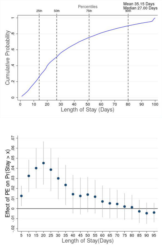
Figure C.2: Patient Length of Stay
A: Length of Stay Distribution
B: Effect on Length of Stay
Note: This figure presents plots relating to patient length of stay. Panel A presents a histogram of the cumulative
probability for patient length of stay (in days). Panel B presents estimates for effect of private equity on shift
in distribution of length of stay. For Panel B, the x-axis represents the length of stay (in days) and the y-axis
represents the coefficient β for the probability that length of stay is greater than the number of days as specified
on the x-axis. Each blue point in the figure is obtained by separately estimating β using Equation (2) with the
dependent variable being an indicator which equals one if length of stay for patient is greater than corresponding
value on x-axis. As an example, the dependent variable for the first point (x = 5 days) is an indicator which equals
one if patient length of stay is greater than 5 days. The equation is estimated via 2SLS where independent variable
is an indicator for the patient being admitted to a PE nursing home, instrumented by differences in distance to the
nearest PE and non-PE facility. Regressions include facility and patient HRR x Year fixed effects, and patient risk
controls. Patient risk controls include age, race, gender, marital status, indicators for 17 pre-existing conditions
used to compute the Charlson Index, and an indicator if patients are dual eligible. Standard errors are clustered by
facility.
62
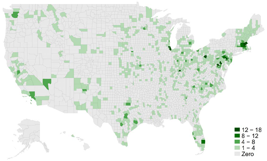
Figure C.3: Location of Private Equity Targets
Note: This figure presents the number of facilities bought by PE firms in each county over the period 2004–2015.
We identified 1,674 such facilities.
63
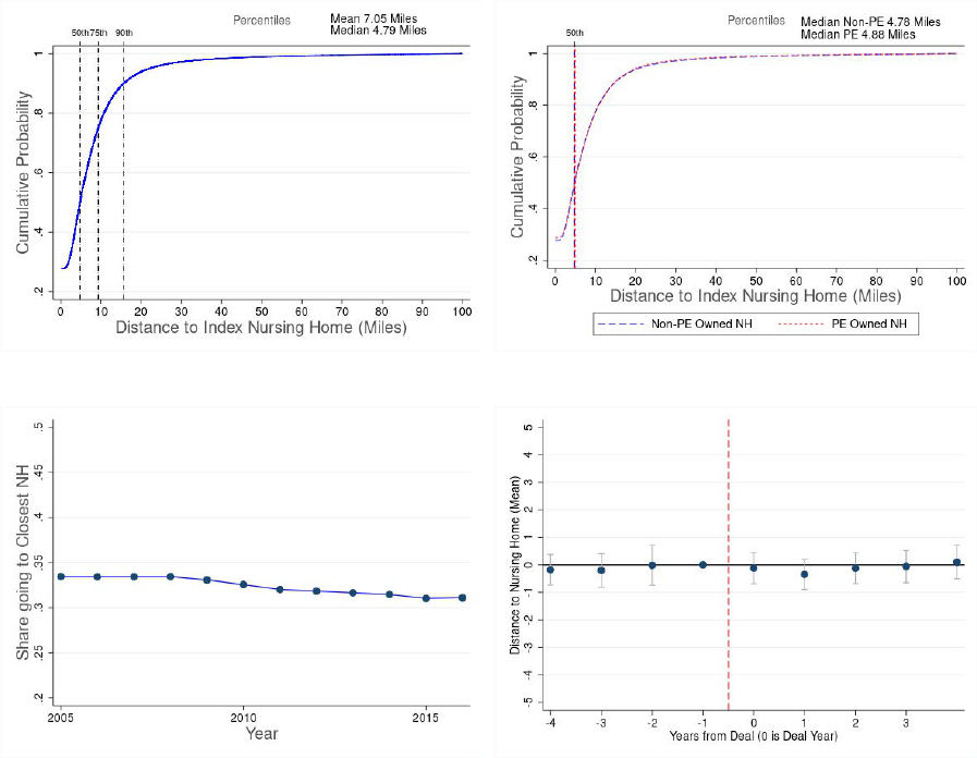
Figure C.4: Patient Distance to Nursing Home
A: CDF: All Patients B: CDF: PE vs. Non-PE Patients
C: Trendline: Share going to Closest Nursing Home D: Event Study: PE Acquisition
Note: This figure provides descriptives on patient zip code distance to index nursing home zip code. Panels A and
B present CDFs of the distance from patient zip code to index nursing home zip code. Panel A presents the CDF
pooling PE and non-PE patients together. It also identifies the median, 75th and 90th percentile values. Panel B
presents the CDFs separately for PE and non-PE patients, and their respective median values. Panel C presents the
annual trendline for the share of patients going to their closest nursing home. Panel D presents the event study of
the mean patient distance around a PE acquisition. Each point in the figure represents the coefficient β
s
obtained
by estimating Equation (5) as discussed in Section 6. The model is fully saturated, including coefficients for all
years except Year = -1, which is the omitted point, but we plot only years -4 to 4. The model includes facility and
HRR x year fixed effects, patient mix, and market controls. Standard errors are clustered by facility.
64
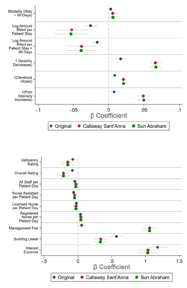
Figure C.5: OLS Results with Alternative Estimators
A: Patient-Level Outcomes
B: Facility-Level Outcomes
Note: This figure presents reports coefficients and 90% confidence intervals for the Callaway and Sant’Anna
(2021) and Sun and Abraham (2021) alternative estimators for all outcomes. Panel A shows the five patient-
level outcomes, while Panel B shows the nine facility-level outcomes. These address potential bias in the size or
direction of coefficients from staggered differences-in-differences models.
65
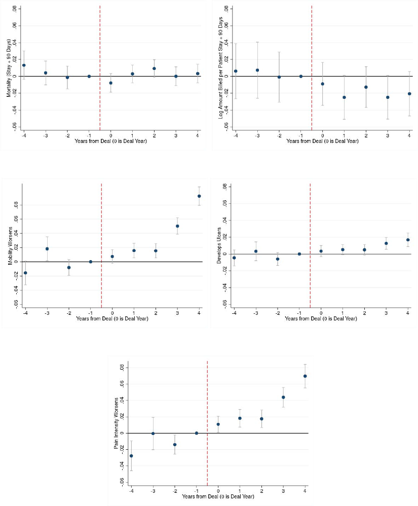
Figure C.6: Patient Outcome Measures
A: Mortality (Stay + 90 Days) B: Log Amount Billed (Patient Stay + 90 Days)
C: 1(Mobility Decreases) D: 1(Develops Ulcers)
E: 1(Pain Intensity Increases)
Note: This figure presents event studies on patient outcome measures around the time a nursing home experiences
a PE buyout. These models were estimated on collapsed facility-year level data using an event study version of
Equation (1). The model is fully saturated, including coefficients for all years except Year = -1, which is the
omitted point, but we plot only years -4 to 4. Panels A and B present results on the share of patients dying within
90 days of discharge from the index stay, and total amount billed over the 90-day episode including the index stay
(2016$). Panels C to E present results for MDS assessment based outcomes - the facility level mean for indicators
for decrease in patient mobility, developing/worsening pressure ulcers, and increase in pain intensity respectively.
Spending is winsorized at the 1% and 99% level. Standard errors are clustered by facility.
66
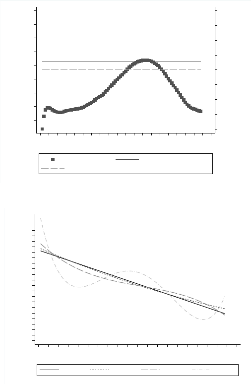
Figure C.7: MTE Specification Checks
0.000
0.005
0.010
0.015
0.020
0.025
0.030
0.035
0.040
Treatment effect
0.000
0.005
0.010
0.015
0.020
0.025
0.030
0.035
0.040
IV weights
0.0 0.1 0.2 0.3 0.4 0.5 0.6 0.7 0.8 0.9 1.0
Unobserved resistance to treatment
IV weights IV-weighted MTE (.023)
IV-2SLS (.02)
A: IV estimate
-0.03
-0.02
-0.01
0.00
0.01
0.02
0.03
0.04
0.05
0.06
0.07
MTE
0.0 0.1 0.2 0.3 0.4 0.5 0.6 0.7 0.8 0.9 1.0
Unobserved resistance to treatment
Baseline 3rd order 4th order 5th order
B: Order of polynomial
Note: This figure presents results from specification checks pertaining to the Marginal Treatment Effects (MTE)
analysis. Panel A tests robustness of the slope of the MTE curve to using different orders of polynomials. Panel B
presents the weights to compute the weighted average equivalent of the 2SLS estimate (left axis) and the weighted
average value (solid line, right axis). The figure also indicates the 2SLS estimate (dashed line) presented in the
main results. Section 5.2 presents details of the MTE estimation.
67
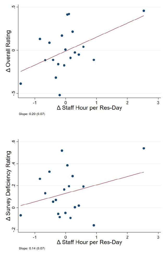
Figure C.8: Staff Availability and Five Star Ratings
A: Overall Rating
B: Deficiency Rating
Note: This figure presents scatter plots of changes in total staff hours available per patient day in the three years
post-PE buyout versus three years pre-buyout on the X-axis, against changes in CMS Five-star rating over the
same period on the Y-axis. Panel A presents overall rating, and Panel B presents survey based deficiency ratings.
The data was collapsed into 20 equal sized bins and we plot the means in each bin. The figures also present fitted
lines for these plots obtained using linear regressions on the underlying data. Each plot also presents the slope
coefficient with standard error.
68
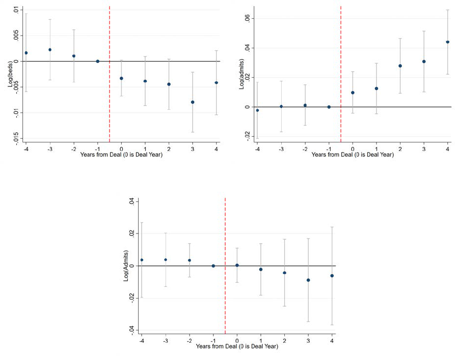
Figure C.9: Patient Volume
A: Log Beds - Facility B: Log Admissions - Facility
C: Log Admissions - Market (HRR)
Note: This figure presents event studies on facility characteristics around the time a nursing home experiences a
PE buyout. Each point in the figures represents the coefficient β
s
obtained by estimating Equation (5) as discussed
in Section 6. The model is fully saturated, including coefficients for all years except Year = -1, which is the omitted
point, but we plot only years -4 to 4. Panels A and B present results on the log of beds and admissions at the facility
level, and Panel C on log admissions at the market level (HRR). All models – except when studying market-level
volume – include facility and year fixed effects, patient mix, and market controls, as described in Section 6.1. All
dependent variables are winsorized at 1% and 99% levels. Standard errors are clustered by facility.
69

Table C.1: Top 5 Private Equity Deals
Sr. Target Private Equity Deal Number of
No. Name Firm(s) Year Facilities
1 Genesis Healthcare Formation Capital, JER Partners 2007–15 327
2 Golden Living Fillmore Capital Partners 2006 321
3 Kindred Healthcare Signature Healthcare, Hillview Capital 2014 150
4 HCR Manorcare Stockwell Capital, The Carlyle Group 2007–18 145
5 Mariner Healthcare Fillmore Capital Partners 2004 95
Note: This table presents some details on the top 5 PE deals in our sample, ordered by the number of unique
nursing home facilities involved in the deal. This represents the number of facilities we were able to identify and
match in our administrative data, the actual number of facilities in the deal may have been different. We set the PE
indicator to turn on in the year following the deal year. If a closing year is mentioned, it implies the PE investors
exited or went public in that year. Accordingly, we turn off the PE indicator in the closing year.
70

Table C.2: Complier Characteristics
Observations Coefficient (Std. Errors) Ratio
Full Sample 4,231,356 -0.0554*** (0.003)
A. Risk
Low Risk 3,073,198 -0.0543*** (0.003) 0.98
High Risk 1,157,836 -0.0582*** (0.003) 1.05
B. Gender
Male 1,547,356 -0.0570*** (0.003) 1.03
Female 2,683,713 -0.0545*** (0.003) 0.98
C. Marital Status
Unmarried 2,757,830 -0.0550*** (0.003) 0.99
Married 1,473,244 -0.0556*** (0.003) 1.00
D. Beneficiary Zip Income
Income < Median 2,114,861 -0.0639*** (0.004) 1.15
Income > Median 2,115,962 -0.0500*** (0.004) 0.90
E. Race
White 3,687,422 -0.0577*** (0.003) 1.04
Other 543,185 -0.0386*** (0.003) 0.70
Note: This table presents first stage equivalent estimates of the 2SLS for various patient
subsamples. We present the coefficient β, obtained by estimating the equation PE
i
= α
j
+
α
m,t
+ β 1(DD
i
> Median) +
i
. 1(DD
i
> Median) is an indicator for patient i’s differential
distance to the nearest PE-owned facility being greater than the median value. The model
includes facility j and patient HRR x year fixed effects, but no other controls. We divide
the sample by risk, gender, marital status, income in patient zip code, and race. We also
present the ratio of the coefficient obtained for each subsample to that for the full sample.
Standard errors are clustered by facilities. *p < .1, ** p < .05, *** p < .01.
71

Table C.3: Mortality Costs
(1) (2)
Male Female
A: IV estimates
1(PE) 0.0201* 0.0186**
(0.012) (0.008)
Observations 1,547,356 2,683,713
Y-Mean 0.23 0.16
F-Stat 246 236
B: Placebo
1(PE) 0.0088 -0.0015
(0.006) (0.005)
Observations 1,315,632 2,395,244
Y-Mean 0.25 0.17
F-Stat 600 574
C: Calculations
Number of Patients in PE Facilities 435,035 741,838
Additional Deaths 8,744 13,798
Total Lives Lost 22,542
Mean Life Expectancy 6.8 8.2
Additional Loss in Person Years 59,203 113,190
Total Person Years Lost 172,393
Value of Life Year (2016 $) 130,000
Total Cost (2016 $) 22.41 Billion
Note: This table presents estimates of additional deaths, life-years lost, and the associated
cost using standard estimates of statistical value of a life-year due to PE ownership of
nursing homes. Panel A presents the coefficient β obtained by estimating Equation (3)
by 2SLS. The independent variable is the indicator for a patient being admitted to a PE
nursing home, instrumented by differences in distance to the nearest non-PE and PE nursing
home. The outcome variable is an indicator for patient death within 90 days of discharge
from the index stay. Panel B presents a placebo analysis for this patient subsample using
the same approach as for the whole sample, as presented in Table 2. All models include
facility and patient HRR x year fixed effects and the usual patient risk controls as in the
main specification. Standard errors are clustered by facility. Panel C presents calculations
to estimate lives, life-years lost and total cost based on Panel A coefficients. We calculate
average life expectancy at discharge (by gender) using the observed distribution of lifespans
for Medicare patients. For patients still alive at the end of our sample, we assign a year of
death based on patient gender and age using Social Security actuary tables. We adjust
downward the resulting life expectancy to account for the fact the decedents tend to be
older than the average nursing home patient (about two years). *p < .1, ** p < .05, ***
p < .01.
72

Table C.4: Effects By Differential Distance
Minimum Differential Distance Basis Patient Zip (in Miles)
(1) (2) (3) (4) (5) (6)
Base Sample -1 <DD < 1 DD > 20 DD > 30 DD > 40 DD > 50
First Stage
F-Stat 259.34 0.28 17.36 5.88 0.25 0.46
P-Value (0.00) (0.76) (0.00) 0.00 (0.78) (0.63)
Reduced Form
F-Stat 5.15 1.32 0.04 0.42 1.39 0.18
P-Value (0.01) (0.27) (0.96) (0.65) (0.25) (0.84)
Observations 4,054,602 200,553 821,687 417,476 220,067 105,820
Note: This table presents the F-statistic and p-value from the joint test of significance on the differential distance
coefficients in the first stage and reduced form (with 90-day mortality as the outcome) models for different patient
sub-groups. Column 1 presents estimates from our main sample, where the differential distance (DD) is less than
20 miles in magnitude (−20 ≤ DD ≤ 20). Column 2 onwards we replicate the first stage and reduced form models
on different sub-groups based on the differential distance values. For example, in Column 2 we only retain patients
residing in zip codes such that their distances to PE and non-PE facilities are very similar (differ by < 1 mile).
Column 3 only retains patients located in zip codes that are at least 20 miles further away from a PE facility relative
to a non-PE facility. Columns 4, 5, and 6 are similarly defined. All models include patient controls, facility, and
HRR × year fixed effects. Standard errors are clustered by facility.
73

Table C.5: Mortality Effects by Duration
(1)
(2) (3) (4) (5)
(Stay + 15 Days) (Stay + 30 Days) (Stay + 60 Days) (Stay + 90 Days) (Stay + 365 Days)
1(PE)
0.0095* 0.0109* 0.0186*** 0.0195*** 0.0245***
(0.006) (0.006) (0.007) (0.007) (0.008)
Observations 4,231,356 4,231,356 4,231,356 4,231,356 4,231,356
Y-Mean 0.10 0.13 0.16 0.18 0.25
F-Stat 242.7 242.7 242.8 242.7 242.7
Coefficient/ Y-Mean 10% 9% 12% 11% 10%
Note: This table presents estimates of the relationship between PE ownership and patient mortality. Each cell
presents the coefficient β obtained by estimating Equation (3) by 2SLS. The independent variable is an indicator
for the patient being admitted to a PE nursing home, instrumented by differences in distance to the nearest PE and
non-PE facility. We present effects for mortality at different durations - patient death within 15, 30, 60, 90, and 365
days of discharge from the index stay. All regressions include facility and patient HRR x year fixed effects, and
patient risk controls. Patient risk controls include age, race, gender, marital status, indicators for 17 pre-existing
conditions used to compute the Charlson Index, and an indicator for dual eligibility. Standard errors are clustered
by facility. *p < .1, ** p < .05, *** p < .01.
74

Table C.6: Patient Sourcing & Discharge
A: Upstream (Mortality from Hospital)
HRR Dartmouth HSA County
(1) (2) (3)
Mortality Mortality Mortality
(Stay + 90 Days) (Stay + 90 Days) (Stay + 90 Days)
1(PE) -0.004 -0.001 0.001
(0.002) (0.002) (0.002)
Observations 504,376 504,376 504,376
Y-Mean 0.16 0.16 0.16
B: Upstream (Discharge from Hospital)
HRR Dartmouth HSA County
(1) (2) (3)
Discharge to Discharge to Discharge to
Nursing Home Nursing Home Nursing Home
1(PE) 0.000 0.002 0.001
(0.002) (0.002) (0.002)
Observations 29,900,000 29,900,000 29,900,000
Y-Mean 0.14 0.14 0.14
C: Downstream (Discharge from Nursing Home)
(1) (2) (3)
Discharge to Discharge to Discharge to
Home Facility Other
1(PE) 0.014 -0.0178* 0.004
(0.011) (0.010) (0.009)
Observations 4,231,356 4,231,356 4,231,356
Y-Mean 0.57 0.26 0.17
F-Stat 243 243 243
Note: This table presents estimates for effects on PE on patient admissions from hospitals to nursing homes and
on discharge from nursing homes. Panels A and B presents results for Upstream facilities - the 90-day mortality
for AMI patients admitted to hospitals, and discharge from hospitals to nursing homes, respectively. We present
the coefficient β, obtained by estimating the equation Y
i, j,t
= α
j
+ α
t
+ β PE
j,t
+ X
i
+
i
. PE
j,t
is an indicator
whether hospital j’s market has PE owned nursing home (=1 if PE-owned, 0 otherwise) in year t. Column 1
defines markets based on HRR, Column 2 on HSA, and Column 3 on County. The model includes hospital j and
year fixed effects, and controls for patient risk: age, gender, and indicators for 17 pre-existing conditions used to
compute the Charlson score. Standard errors are clustered by hospitals. Panel C presents results for Downstream
Channel - discharge from nursing homes to different facilities. Each cell presents the coefficient β obtained by
estimating Equation (3) by 2SLS. The independent variable is an indicator for the patient being admitted to a
PE nursing home, instrumented by differences in distance to the nearest PE and non-PE facility. We present
probability of discharge to patient residence, facility (including hospitals, long stay nursing homes and hospice),
and all other discharges. All regressions include facility and patient HRR x year fixed effects, and patient risk
controls. Patient risk controls include age, race, gender, marital status, indicators for 17 pre-existing conditions
used to compute the Charlson Index, and an indicator for dual eligibility. Standard errors are clustered by facility.
*p < .1, ** p < .05, *** p < .01.
75

Table C.7: Effects on Quality by Share Revenue from Medicare
A:
Five Star Rating
Deficienc
y Rating Overall Rating
Medicare < Median
Medicare > Median Medicare < Median Medicare > Median
(1)
(2) (3) (4)
1(PE)
0.027 -0.120*** -0.033 -0.101**
(No Control) (0.071) (0.043) (0.071) (0.042)
1(PE) 0.025 -0.125*** -0.036 -0.107**
(With Control) (0.071) (0.043) (0.071) (0.042)
Observations 53,615 58,102 53,615 58,102
Y-Mean 2.8 2.8 3.1 3.0
Note: This table presents estimates of the relationship between PE ownership and nursing home quality as
measured by the Five Start ratings. We repeat the models in Table 8 Panel A, but divide the sample by whether the
nursing home’s revenue from Medicare is above or below the median. Each cell presents the coefficient β obtained
by estimating Equation 4. The independent variable is an indicator for whether a nursing home is PE-owned (=1
if PE-owned, 0 otherwise) starting in the next year from the deal announcement date. All models include facility
and year fixed effects. All variables are winsorized at 1% and 99% levels. Standard errors are clustered by facility.
*p < .1, ** p < .05, *** p < .01.
76

Table C.8: Robustness: Facility-Level Outcomes
A:
Five Star Rating
(1)
(2)
Deficiency Overall
Rating Rating
1.
Chain Controls
1(PE) -0.077** -0.082**
(0.036) (0.028)
2. W/O Top 2 Deals
1(PE) -0.145*** -0.209***
(0.050) (0.042)
Observations 111,728 111,728
Y-Mean 2.8 3.1
B:
Staff Per Patient Day
(1)
(2) (3) (4)
All Staff Nurse Assistant Licensed Nurse Registered Nurse
1.
Chain Controls
1(PE) -0.045*** -0.062*** -0.024*** 0.039***
(0.017) (0.010) (0.006) (0.005)
2. W/O Top 2 Deals
1(PE) -0.097*** -0.096*** -0.027*** 0.032***
(0.026) (0.015) (0.009) (0.008)
Observations 227,254 227,254 227,254 227,254
Y-Mean 3.4 2.2 0.8 0.4
C:
Log Financials
(1)
(2) (3)
Management Fee Building Lease Interest Expense
1.
Chain Controls
1(PE) 0.056* 0.570*** 1.179***
(0.032) (0.061) (0.096)
2. W/O Top 2 Deals
1(PE) 0.036 0.816*** 2.041***
(0.051) (0.102) (0.160)
Observations 196,880 196,900 196,918
Y-Mean 0.2 0.4 0.3
Note: This table presents robustness tests on the estimates of the relationship between PE buyouts and Five Star
ratings, nurse availability, and financials. The corresponding main results are presented in Table 8. Each cell
presents the coefficient β obtained by estimating Equation (4) with a different outcome. The independent variable
is an indicator for whether a nursing home is PE-owned (=1 if PE-owned, 0 otherwise) starting in the next year
from the deal announcement date. We control for a chain indicator in the first row and remove the top 2 deals by
size in the second row. We do not present results limiting to the Top 5 deals as Five Star ratings are only available
post-2009, and 4 Top 5 deals occurred before 2009. All models include facility and year fixed effects. All variables
are winsorized at 1% and 99% levels. Standard errors are clustered by facility. *p < .1, ** p < .05, *** p < .01.
77

Table C.9: Goodman-Bacon Decomposition: Facility-Level Outcomes
A:
Five Star Rating
(1)
(2)
Deficiency Overall
Rating Rating
Ov
erall
1(PE) -0.0384 -0.1839***
(0.059) (0.062)
Never PE vs. Timing
1(PE) -0.0395 -0.1774
Weight 0.89 0.89
Always PE vs. Timing
1(PE) -0.0342 -0.2066
Weight 0.10 0.10
Observations 68,363 68,363
Y-Mean 2.8 3.1
B:
Staff Per Patient Day
(1)
(2) (3) (4)
All Staff Nurse Assistant Licensed Nurse Registered Nurse
Ov
erall
1(PE) -0.0337*** -0.0693*** -0.0310*** 0.0602***
(0.012) (0.009) (0.004) (0.003)
Never PE vs. Timing
1(PE) -0.0373 -0.0725 -0.0321 0.0607
Weight 0.97 0.97 0.97 0.97
Always PE vs. Timing
1(PE) 0.1304 0.0347 -0.0610 0.1773
Weight 0.00 0.00 0.00 0.00
Observations 148,239 148,239 148,239 148,239
Y-Mean 3.4 2.2 0.8 0.4
C:
Log Financials
(1)
(2) (3)
Management Fee Building Lease Interest Expense
Ov
erall
1(PE) 0.8278*** 0.3761*** 0.9978***
(0.020) (0.028) (0.026)
Never PE vs. Timing
1(PE) 0.8414 0.3747 1.0065
Weight 0.97 0.97 0.97
Always PE vs. Timing
1(PE) 0.9584 0.9298 2.8155
Weight 0.00 0.00 0.00
Observations 131,431 131,438 131,445
Y-Mean 0.2 0.4 0.3
Note: This table presents heterogeneity in component estimates for our key aggregate outcomes. obtained by
following Goodman-Bacon (2021) and using the main specification (Equation 4). The corresponding main results
are presented Table 8. For this analysis we had to limit the sample to ensure a balanced panel, which affected the
overall estimates slightly. Each cell presents the coefficient β obtained by estimating Equation (4) with a different
outcome. The independent variable is an indicator for whether a nursing home is PE-owned (=1 if PE-owned,
0 otherwise) starting in the next year from the deal announcement date. We show the overall effect in the first
row, the coefficient and weight of Never PE vs. staggered PE indicator in the second row, and the coefficient and
weight for Always PE vs staggered PE indicator in the third row. All variables are winsorized at 1% and 99%
levels. Standard errors are clustered by facility. *p < .1, ** p < .05, *** p < .01.
78

Table C.10: Patient Volume
Facility Level Market Level
(1) (2) (3)
Log Log Log
Beds Admissions Admissions
1(PE) -0.006* 0.030*** 0.001
(No Control) (0.003) (0.009) (0.015)
1(PE) -0.006* 0.033*** -0.003
(With Control) (0.003) (0.009) (0.013)
Observations 227,254 227,254 5,364
Y-Mean 4.6 4.8 12.4
Note: This table presents estimates of the relationship between PE ownership and patient volume. Each cell
presents the coefficient β obtained by estimating Equation (4) with a different outcome. The independent variable
is an indicator for whether a nursing home is PE-owned (=1 if PE-owned, 0 otherwise) starting in the next year
from the deal announcement date. We present results on the log number of beds, log number of admissions in
facility, and log number of admissions at HRR level. The bottom row presents the results including controls,
which consist of market-level and patient mix controls, as described in Section 6.1. All models include facility
and year fixed effects. All variables are winsorized at 1% and 99% levels. Standard errors are clustered by facility.
*p < .1, ** p < .05, *** p < .01.
79

Table C.11: Effects on Quality & Staffing by Fund Characteristics
(1) (2) (3) (4)
Observations Mean Coefficient (Std. Errors)
A. Overall Five Star Rating
1. PE Specialization
1(PE) 111,239 3.07 0.018 (0.051)
1(PE) X 1(Health Specialist PE) -0.183** (0.074)
2. Total Liability ($ Mns)/Bed
1(PE) 103,402 3.07 -0.056 (0.039)
1(PE) X Total Liability/ Bed -0.261* (0.135)
3. PE Vintage
1(PE) 103,340 3.07 0.286* (0.161)
1(PE) X Fund Age -0.051 (0.037)
B. All Staff Per Patient Day
1. PE Specialization
1(PE) 226,300 3.44 -0.018 (0.018)
1(PE) X 1(Health Specialist PE) -0.083** (0.036)
2. Total Liability ($ Mns)/Bed
1(PE) 196,803 3.45 0.050*** (0.018)
1(PE) X Total Liability/ Bed -0.958*** (0.204)
3. PE Vintage
1(PE) 210,816 3.46 0.035 (0.046)
1(PE) X Fund Age -0.021 (0.013)
Note: This table presents heterogeneity in overall quality and staffing outcomes. Column 1 presents the sample
size and Column 2 presents the mean of the dependent variable. Columns 3 and 4 present the corresponding
coefficient β and its standard error. The independent variable is an indicator for whether a nursing home is PE-
owned (=1 if PE-owned, 0 otherwise) starting in the next year from the deal announcement date. This variable
is interacted with different fund characteristics in each panel, and Column 3 presents the coefficient β
1
(on an
indicator whether nursing home is PE-owned) and β
2
(on the indicator whether nursing home is PE-owned
interacted with fund characteristics) obtained by estimating a triple difference version of Equation (4). We do
not show other interactions for brevity. Panel A shows the impact on overall five star ratings, and Panel B shows
the impact on total staff per patient day. We interact the indicator whether nursing home is PE-owned with an
indicator for whether the PE fund specializes in Healthcare deals in rows A1 and B1, the total liability of the
nursing home ($ Millions) per bed in rows A2 and B2, and the age of the fund in the year the deal happens in rows
A3 and B3. Observations vary slightly by the characteristic of interest because liability amounts are not reported
for some facilities and we were not able to determine the fund vintage for a few deals. All variables are winsorized
at 1% and 99% levels. Standard errors are clustered by facility. *p < .1, ** p < .05, *** p < .01.
80
