
19
th
World Conference on Non-Destructive Testing 2016
1
License:
http://creativecommons.org/licenses/by/3.0/
Modelling the IMPOC Response for Different
Steel Strips
Anastassios SKARLATOS
1
, Christophe REBOUD
1
, Tomas SVATON
1
,
Ane MARTINEZ-DE-GUERENU
2
, Thomas KEBE
3
, Frenk VAN DEN BERG
4
1
CEA Commissariat à l'Energie Atomique, Gif-sur-Yvette, France
2
CEIT, San Sebastián, Spain
3
thyssenkrupp Steel Europe AG, Duisburg, Germany
4
Tata Steel, IJmuiden, Netherlands
Contact e-mail: a[email protected]
Abstract. The IMPOC system is used in steel industry for the assessment of steel strip
mechanical properties by means of electromagnetic measurements [1]. The
development of a simulation tool for the calculation of the system’s response is
expected to enhance the device signals’ interpretation, to contribute to the
understanding of spurious effects like the speed of the strip and to aid the
improvement of the system’s hardware as well as the inspection process.
The IMPOC signals are derived from measurements of the strip remanent field
resulting by a strong magnetization impulse. Thus, to proceed to quantitative
calculation of the system’s response one needs to solve the Maxwell’s equations in
the presence of a non-linear and hysteretic medium.
Prerequisite for this calculation is the detailed knowledge of the full family of
hysteresis curves describing the B-H behaviour of the material, which is an input
parameter to the electromagnetic solver. They can be obtained either by direct
measurement or using parametric models. In the second case experimental data is still
required in order to estimate the parameters of the considered model that best fit the
experimental curves.
In this contribution, numerical simulations of the IMPOC impulse response using
an electromagnetic solver based on the finite integration technique (FIT) will be
presented for dual phase (DP) steels. The hysteresis curves of both grades have been
obtained experimentally on strip samples provided by thyssenkrupp Steel Europe and
Tata Steel using two different measuring techniques, that is, Epstein frame and
ferromagnetic yoke measurements. All measurements have been carried out for both
parallel and transversal to the strip rolling direction. The experimental data are used
either directly (with appropriate interpolation) or as reference for fitting the Jiles-
Atherton and the Mel'gui parametric hysteresis models. Moreover, simulation results
using the B-H curves for the two directions (longitudinal and transversal) allow us to
assess the importance of the anisotropy effect as well as its impact to the system’s
response.
This work has been carried out in the context of the European project Product
Uniformity Control (PUC), funded by the RFCS program.
More info about this article: http://ndt.net/?id=19415
2
1. Introduction
1.1 Description of the IMPOC system
The IMPOC-system (Impulse Magnetic Process Online Controller) [1,2] is an online
measurement device which has been implemented by a number of major steel producers in
Europe [3,4] in order to monitor the techno-mechanical properties, in particular tensile
strength and yield strength, of the steel strip over its length during production. It is distributed
under license from EMG Automation Company in Wenden, Germany [5].
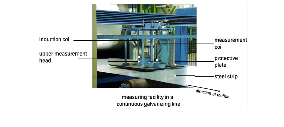
The system consists of two measuring heads with induction coils and a magnetic field
sensing probe. The heads are arranged opposed with a gap of 50 mm. In between the steel
strip is moving such that the clearance of each head with respect to the strip is approximately
25 mm. Fig. 1 shows a photograph of an IMPOC head in a continuous galvanizing line
operation position. The lower head is hidden behind the steel strip.
At each measurement a current pulse through both induction coils induces high
magnetic fields at the steel strip which magnetizes the steel locally into saturation. After the
magnetic pulse a residual magnetization remains in the strip which gives rise to magnetic
stray fields of the steel strip. About 70 mm further downstream, the magnetised spot in the
moving steel strip passes magnetic field gradiometer sensors which probe the magnetic stray
fields. The maximum of the measured signal is stored. By averaging the signals of upper and
lower head the so-called IMPOC value is generated. This makes the system relatively
independent of pass line variations within a range of ± 5 mm.
1.2 Motivation for this work
In the framework of the European PUC project [6], a measurement model is established for
the IMPOC system to enhance the interpretation of the data and broaden its applicability
scope to new steel grades. Past work [7] has shown that the measured IMPOC value can be
influenced by strip speed, material thickness and other measurement conditions. These
sensitivities are often coupled and sometimes even steel-grade dependent. Although these
effects can partly be compensated using calibration procedures based on statistical analysis
of many coil data, this is a labour-intensive and time consuming job, causing a delay in return
on investment. It is believed that the calibration of the IMPOC and the interpretation of the
data will accelerate by the construction of an accurate, physics-based model of the
instrument.
Fig. 1. Photograph of the IMPOC-system measuring head in a continuous galvanizing line at thyssenkrupp Steel
Europe.

3
1.3 General approach
The IMPOC measurement model is a transient pseudo-3D electromagnetic model, involving
the solution of the Maxwell's equations employing a non-linear and hysteretic magnetic
constitutive relation. In the low-frequency regime, that is neglecting the displacement
current, and ignoring the stationary electric charges on the conductors’ interfaces, the
governing equations of the problem read:
(1)
(2)
where is the excitation current, and stands for the electric conductivity of the medium.
The magnetic flux density B and the magnetic field H are related via the magnetic constitutive
relation B(H), which in the case of ferromagnetic material is a non-linear, hysteretic curve.
In our modelling, the B(H) curves are assumed constant over the relevant material volume
and are either retrieved from experiments or theoretical calculations from other project
partners (e.g. [8,9]) and parameterised using a procedure that has been detailed in [10].
2. Numerical evaluation of the IMPOC response
In order to calculate the IMPOC system response, we need first to solve the non-linear
hysteretic field problem during the excitation time, and then the thus computed remanent
field must be propagated to the receiver. For the solution of the former, a numerical scheme
based on the finite integration technique (FIT) [11] has been developed, whereas an efficient
analytical propagator is adopted for the latter in order to avoid the introduction of numerical
noise linked to the computational grid in the calculation of the final signal.
2.1 Description of the solution algorithm
Since we are interested in calculating the transient field response, direct integration in the
time domain by applying a time stepping scheme is the most pertinent approach. A non-linear
problem has thus to be treated at each time step, which is solved iteratively via successive
linearizations. The hysteretic character of ferromagnetic media introduces an additional
degree of complexity, and, accordingly, an additional step in the solution algorithm, which
is responsible for performing the switching between the different branches at the extrema of
the excitation. This general solution strategy for the non-linear, hysteretic problem is
illustrated in the form of a block diagram in Fig. 2.
2.2 Solution of the linearized problem using the FIT
According to the general scheme of the FIT method, Maxwell's equations are discretized
using a set of dual, mutually orthogonal grids
. As state variables for the electric field and
the magnetic vector potential we use their integrated values along the edges of the primary
field, , whereas the corresponding integrals along the dual grid edges stand for the state
variable for the magnetic field,
. The scheme is completed by the flux associated state
variables,
, which stand for the integrated current and magnetic flux densities integrated
over the facets of the primary and the dual grid, respectively [11]. With the above definitions,
the constitutive relations for the electric (eddy) current and the magnetic field read:

4
Fig. 2. General iterative scheme for the treatment of non-linear, hysteretic electromagnetic problem in the
time domain.
(3)
(4)
with
and
diagonal matrices of the discretized distribution for the electrical
conductivity σ and the magnetic reluctivity ν, respectively.
The diffusion equation for the magnetic vector potential after the application of the
FIT discretization scheme becomes
(5)
where
are topological matrices, associated with the primary and the dual
grid,
respectively, and which form the analogous of the continuous curl operator to the grid vector
space, and
stands for the excitation current.
In case of ferromagnetic media, the magnetic constitutive equation is a non-linear
equation since the reluctivity matrix
depends on the magnetic field. There are in general
two well established approaches for addressing the non-linear problem: the Picard-Banach,
or fixed point, method and the Newton-Raphson method. Both approaches are based on an
iterative procedure, which consists in linearizing the initial problem and building a sequence
of successive approximations until a convergence criterion is satisfied. The main difference
of the methods relies on the way that the linearized problem is established. If, in addition, a
first order backward differentiation scheme (also known as Euler scheme) is adopted for the
discretization of the time derivatives, both non-linear approaches can be written in the
following fashion [12]
(6)

5
for the (n+1)-th timestep and the i-th non-linear iteration, with
, and
the linearized reluctivity matrix. In the case of the Picard-Banach approach, the
constitutive relation is written as:
(7)
where
is the reluctivity of the free space and stands for the discretized magnetisation.
The linearized material matrix in this case is
. When the Newton-Raphson method is
applied,
with
being the Jacobian of
, namely [12]
(8)
which turns out to be the matrix of the differential reluctivity, i.e. the slope of the
curve
at the point of operation. Notice that
remains invariable, whereas
has to be
recalculated at each iteration.
The two iterative methods are complementary in terms of the converge behaviour.
More precisely, whereas the Picard-Banach scheme is always convergent albeit slow, the
Newton-Raphson method benefits a quadratic convergence speed but it may stagnate. Thus,
by combining them we can obtain a convergent scheme significantly faster than the one of
the Picard-Banach approach. Such a hybrid scheme based on an optimization algorithm is
proposed in [12]. In the present work, a simpler hybridization is followed by switching from
the Picard-Banach to the Newton method when the relative error between two successive
iterations falls below a fixed threshold (
in this case).
2.3 Calculation of the magnetic field at the receiver using an analytic propagator
The relatively large distance of the IMPOC receiver from the inspected piece makes the
calculation of the final signal sensitive to the grid noise, since all the air region between piece
and receiver has to be discretised. An alternative to the direct extraction of the field value at
the receiver position from the FIT numerical solution is to propagate analytically the solution
for the remanent field on the piece interface via an analytic operator involving the Green’s
function of the free space. The main idea in this approach consists to consider the normal
magnetic induction component on the piece surface
as an equivalent magnetic charge
density, which effect at a given observation point in the air region above the piece is given
by the integral
(9)
where 1/
is the Green’s function of the free space, and the integration is carried out
over the interface of the piece .
3. Description of the electromagnetic properties of inspected samples
For the first iteration in model validation, two samples were chosen from two highly different
steel grades, i.e. Interstitial Free (IF) steel and Dual Phase (DP) steel. IF (DP) has relatively
low (high) mechanical yield strength to make it suited for formability (impact-resistance)
applications in car manufacturing. The large span in their mechanical properties stems from
the strong difference in their microstructures, which also causes their B(H) curves to be
distinct.
6
3.1 Experimental data
The samples have been collected from regular production at a hot dip galvanizing line. The
DP steel sample is a HCT600X grade and has a thickness of d=1.39 mm, the IF steel sample
is a DX56 grade with a thickness of 0.82 mm. From the collected sample sheets 12 strips
each are cut in rolling and the transverse direction, respectively, for the magnetic
characterisation.
3.2 Experimental characterization of B(H) curves
The Epstein frame measurement is a standardized method (IEC 60404) to characterize
magnetic losses for soft magnetic materials like grain oriented or non-oriented electric strip.
Its setup is similar to a transformer. The primary outer winding is equipped with a multiple
of 4 sheet strips to form one side of the transformer. The secondary inner winding is used for
detection of the measurement response. The steel strips have dimensions of approx. 300 mm
x 30 mm x sample thickness and are put together such that they form a closed circuit. By
measuring the current of the primary winding and the induced current of the secondary
winding one can deduce the magnetic field and the magnetic inductance, respectively. The
measurements were performed at a frequency of 5 Hz.
Major magnetic B-H loop determination was made using a single sheet tester system
available at CEIT used for material properties and microstructure characterization [13].
Major hysteresis loops were recorded at 0.1 Hz for each steel sample varying the maximum
amplitude of the intensity of the magnetic field applied from H
max
= 190 A/m to
H
max
= 19300 A/m.
3.3 Parametric description
The B-H curve of the considered material is an input variable for the field simulation. It is
obtained either via interpolation from experimentally acquired curves or by means of a
theoretical model. The second case proves to be quite interesting when combined with the
field simulator thanks to its versatility. Note that even in the case where experimental data
exist for a specific material these are usually limited to a very limited number of curves.
Hence some kind of interpolation or theoretical estimation has to be carried out for all the
intermediate curves.
Several models have been proposed in the literature, which provide an estimation of
the material hysteresis curves based on a limited set of parameters. In this work, the scalar
Jiles-Atherton model [14], which is among the most used ones, and the Mel’gui model [15],
which offers a very satisfactory description of the B(H) curves based on a remarkably simple
explicit expression, have been considered. However, in order to estimate the model
parameters that reproduce the curves of the considered material, some kind of fitting must be
carried out between the theoretical model and the available experimental data. This procedure
is particularly simple for the Mel’gui model, since its input parameters are all the physical
quantities like the remanent field, the coercive force, the initial permeability etc., which can
be directly extracted by the experimental curves. For the Jiles-Atherton model the fitting is
more complicated and is realized by means of a numerical optimization technique. More
details on the procedure are given in [10].

7
4. Results and discussion
4.1 Parametric description of B(H) curves
The numerical simulations of the present work were performed for the cold treated dual phase
(DP) steels provided by Tata Steel, and its characteristics are described in the previous
section. For the sake of simplicity no anisotropy was taken into account, with the B(H) curves
in every directions assumed to be the identical with the one measured in the rolling direction.
The Mel’gui model has been fitted to the experimental curves obtained using above
described procedure, and the thus obtained parameters have been used to produce the full
family of curves used by the electromagnetic solver. The result of the fit is shown in Fig. 3
for a number of curves. The agreement between experimental and theoretical curves is very
satisfactory.
Fig. 3. Comparison of the fitted B(H) curves using the Mel’gui model (blue) vs. experimental (red) for a DP
steel.
4.2 Simulation of IMPOC signals
The real IMPOC magnetization coils have a 3D geometry (racetrack coils). Nevertheless,
numerical experimentation using a linear material as well as comparison with measurements
give evidence that a 2D approximation using either a cylindrical coil of a mean diameter
(rotational symmetry) or a long coil of the same width with the narrow side of the IMPOC
racetrack coils (translational symmetry) yield reasonably good results, at least sufficient for
demonstrating the general trends. Notice that the reduction of the original 3D hysteretic
problem to an equivalent 2D one is very beneficial in terms of reduction of the computational
burden, which in the case of the 3D problem can become quite significant. The configuration
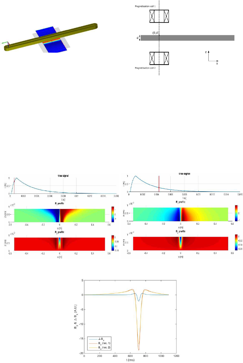
used for the simulation of the IMPOC signals is depicted in Fig. 4. As it can be seen in Fig.
4a, the adopted approximation for the following simulations is that of the translational
symmetry, which has the advantage of allowing us to consider the effect of the coil
movement, and hence to study the effect of the speed (perspective).
8
(a)
(b)
Fig. 4. Considered configuration: (a) 3D view (b) cross-section.
In Fig. 5 two different snapshots of the field profile inside the plate at two
characteristic times are shown: before the excitation peak and during the relaxation time. Fig.
6 illustrates the field response as a function of time at the two sensors of the IMPOC
gradiometer as well as their difference (gradient), which corresponds to the actual IMPOC
measurement. The strip velocity is taken equal to 1 m/s (a mean strip velocity for the
production line). Note that the speed effect has not been taken into account in this simulation,
that is, the strip is assumed to be stationary during the magnetisation phase. The temporal
variation of the measured field and its gradient is a mere result of the strip displacement
during the measuring time window.
Fig. 5. Field profile inside the plate at different time instances.
Fig. 6. Field signals at the receiver. The normal (z) component of the magnetic induction measured at the two
magnetic sensors of the IMPOC gradiometer and their difference (field gradient) are plotted as a function of
time.
5. Conclusion
The IMPOC system is a widely utilized device in steel industry for the assessment of the steel
strip mechanical properties via in-line non-destructive electromagnetic measurements.
9
Accumulated experience by in-situ operation as well as off-line “laboratory-type” conducted
measurements reveal a number of important effects, such as the strip speed effect, influence
of the thickness, etc., which urge quantitative elucidation in order to enhance the signal
interpretation and optimize the tool performance. The development of dedicated simulation
tools, which treat the underlying electromagnetic problem, can offer quantitative answers to
the aforementioned issues and may serve as a valuable aid towards the improvement of both
the device hardware and measuring technique. In the context of the PUC project, a numerical
code has been developed, and the first results (using a simplified version of the real IMPOC
configuration and realistic material characteristics obtained by precise laboratory
measurements) reproduce observed tendencies. Work is under way concerning the fine
tuning of the numerical model. In addition, a program of parametric studies (both
experimental and simulated) is on the way for the systematic study of the most influencing
parameters (like the one of the strip speed and the piece thickness).
Acknowledgement
The research leading to these results has received funding from the European Union’s
Research Fund for Coal and Steel (RFCS) research programme under grant agreement nr.
RFSR-CT-2013-00031.
References
[1] M. Stolzenberg, F. van den Berg, W. Dürr, U. Hofmann, G. Moninger, Stahl und Eisen, Vol. 7, pp 80-90
2012.
[2] V.F. Matyuk, M.N. Delendikh, A.A. Osipov: “The Plant for Pulse Magnetic On-Line Testing of Mechanical
Properties of Rolled Products”, ECNDT 2006, Th. 3.7.5.
[3] T. Kebe, W. Dürr, D. Goureev, G. Reimann, „Einsatz des IMPOC-Verfahrens zur Bestimmung mechanisch-
technologischer Eigenschaften von Bandstahl“, DGZfp annual conference, Bremen, 2011.
[4] M. Bärwald, U. Sommers, M. Biglari, E. Montagna, W. Beugeling, A. Lhoest, “Online quality monitoring
in galvanizing lines”, METEC & ESTAD conference, 2015.
[5] EMG Automation GmbH, Wenden, Germany. http:\\ww.emg-automation.com.
[6] F. van den Berg, P. Kok, H. Yang et al.: “In-line Characterisation of Microstructure and Mechanical
Properties in the Manufacturing of Steel Strip for the Purpose of Product Uniformity Control”, WCNDT-2016
WCNDT-2016, Mo.1.G.
[7] M. Stolzenberg, R. Schmidt, A. Casajus, T. Kebe, M. Falkenstrom, A. Martínez-de-Guerenu, N. Link, H.
Ploegaert, F. van den Berg, A. Peyton, Online material characterisation at strip production (OMC), Technical
Steel Research, 2013, Publications of the European Communities, Luxembourg, ISBN 978-92-79-28961-3,
ISSN: 1831-9424, DOI: 10.2777/77313.
[8]. L. Zhou et al: Magnetic NDT for steel microstructure characterisation – modelling the effect of ferrite grain
size on magnetic properties, WCNDT-2016, Tu.2.H.2
[9]. A. Peyton et al: The Application of Electromagnetic Measurements for the Assessment of Skin Passed Steel
Samples, WCNDT-2016, Th.2.1.4.
[10] P. Meilland et al.: B-H Curves Approximations for Modelling Outputs of Non-Destructive Electromagnetic
Instruments, WCNDT-2016, P91.
[11] M. Clemens and T. Weiland, “Discrete electromagnetism with the finite integration technique”, Progress
Electromagn. Res. (PIER), vol. 32, pp. 65–87, 2001.
[12] I. Munteanu, S. Drobny, T. Weiland and D. Ioan, “Triangle search method for nonlinear electromagnetic
field computation”, COMPEL, vol. 20, No. 2, pp. 417-430, 2001.
[13] M. Soto, A. Martínez-de-Guerenu, K. Gurruchaga, F. Arizti, “A Completely Configurable Digital System
for Simultaneous Measurements of Hysteresis Loops and Barkhausen Noise”, IEEE T. Instrum. Meas., vol. 58,
no. 5, pp. 1746–1755, 2009.
[14] D. C. Jiles and D. L. Atherton, “Theory of ferromagnetic hysteresis”, J. Magn. Magn. Mat., No. 61, pp.
48-60, 1986.
[15] M. A. Mel’gui, “Formulas for describing nonlinear and hysteretic properties of ferromagnets”,
Defektoskopiya, No. 11, pp. 3-10, 1987.
