
Words are not enough! Short text
classification using words as well as
entities
Masterarbeit
von
Qingyuan Bie
Studiengang: Informatik
Matrikelnummer: 1795486
Institut für Angewandte Informatik und Formale
Beschreibungsverfahren (AIFB)
KIT-Fakultät für Wirtschaftswissenschaften
Prüfer: Prof. Dr. Ralf Reussner
Zweiter Prüfer: Prof. Dr. Harald Sack
Betreuer: M.Sc. Rima Türker
Eingereicht am: 29. August 2019

Zusammenfassung
Textklassifizierung, auch als Textkategorisierung bezeichnet, ist eine klassische Aufgabe
in der natürlichen Sprachverarbeitung. Ziel ist es, Textdokumenten eine oder mehrere vor-
definierte Klassen oder Kategorien zuzuordnen. Die Textklassifizierung hat eine Vielzahl
von Anwendungsszenarien.
Herkömmliche Probleme bei der Klassifizierung von Binär- oder Mehrklassentexten wur-
den in der Maschinelles Lernen Forschung intensiv untersucht. Wenn jedoch Techniken des
Maschinelles Lernenes auf kurze Texte angewendet werden, haben die meisten Ansätze
der Standardtextklassifizierung die Probleme wie Datensparsamkeit und unzureichende
Textlänge. Darüber hinaus sind kurze Texte aufgrund fehlender Kontextinformationen
sehr mehrdeutig. Infolgedessen können einfache Textklassifizierungsansätze, die nur auf
Wörtern basieren, die kritischen Merkmale von Kurztexten nicht richtig darstellen.
In dieser Arbeit wird ein neuartiger Ansatz zur Klassifizierung von Kurztexten auf der Ba-
sis neuronaler Netze vorgeschlagen. Wir bereichern die Textdarstellung, indem wir Wörter
zusammen mit Entitäten verwenden, die durch den Inhalt des gegebenen Dokuments re-
präsentiert werden. Tagme wird zuerst verwendet, um benannte Entitäten aus Dokumen-
ten zu extrahieren. Wir verwenden dann das Wikipedia2Vec Modell, um Entitätsvektoren
zu erhalten. Unser Modell wird nicht nur auf vortrainierte Wortvektoren, sondern auch
auf vortrainierte Entitätsvektoren trainiert. Wir vergleichen die Leistung des Modells mit
reinen Wörtern und die Leistung des Modells mit Wörtern und Entitäten. Der Einfluss
verschiedener Arten von Wortvektoren auf die Klassifizierungsgenauigkeit wird ebenfalls
untersucht.
Abstract
Text classification, also known as text categorization, is a classical task in natural lan-
guage processing. It aims to assign one or more predefined classes or categories to text
documents. Text classification has a wide variety of application scenarios.
Traditional binary or multiclass text classification problems have been intensively studied
in machine learning research. However, when machine learning techniques applied to short
texts, most of the standard text classification approaches have the problems such as data
sparsity and insufficient text length. Moreover, due to the lack of contextual information,
short texts are highly ambiguous. As a result, simple text classification approaches based
on words only, can not represent the critical features of short texts properly.
In this work, a novel neural network based approach of short text classification is proposed.
We enrich text representation by utilizing words together with entities represented by the
content of the given document. Tagme is first utilized to extract named entities from
documents. We then utilize Wikipedia2Vec model to get entity vectors. Our model is
trained not only on top of pre-trained word vectors, but also on top of pre-trained entity
vectors. We compare the performance of the model using pure words and the model using
words as well as entities. The impact of different kinds of word vectors on the classification
accuracy is also studied.

INHALTSVERZEICHNIS v
Inhaltsverzeichnis
1 Introduction 1
1.1 Motivation . . . . . . . . . . . . . . . . . . . . . . . . . . . . . . . . . . . . 1
1.2 Contribution . . . . . . . . . . . . . . . . . . . . . . . . . . . . . . . . . . . 2
1.3 Thesis Structure . . . . . . . . . . . . . . . . . . . . . . . . . . . . . . . . . 2
2 Background 3
2.1 Text Classification . . . . . . . . . . . . . . . . . . . . . . . . . . . . . . . 3
2.2 Text Representation (Feature Engineering) . . . . . . . . . . . . . . . . . . 4
2.3 Text Classification (Classifiers) . . . . . . . . . . . . . . . . . . . . . . . . 7
3 Related Work 11
3.1 Text Classification . . . . . . . . . . . . . . . . . . . . . . . . . . . . . . . 11
3.1.1 Vector Representation of Words . . . . . . . . . . . . . . . . . . . . 11
3.1.2 Convolutional Neural Network Feature Extraction . . . . . . . . . . 13
3.1.3 Pre-training & Multi-task Learning . . . . . . . . . . . . . . . . . . 15
3.1.4 Context Mechanism . . . . . . . . . . . . . . . . . . . . . . . . . . . 19
3.1.5 Memory Storage Mechanism . . . . . . . . . . . . . . . . . . . . . . 20
3.1.6 Attention Mechanism . . . . . . . . . . . . . . . . . . . . . . . . . . 20
3.2 Short Text Classification . . . . . . . . . . . . . . . . . . . . . . . . . . . . 21
3.3 Text Classification using Named Entities . . . . . . . . . . . . . . . . . . . 21
4 Wikipedia2Vec and Doc2Vec 23
4.1 Word2vec and Skip-gram . . . . . . . . . . . . . . . . . . . . . . . . . . . . 23
4.2 Wikipedia2Vec . . . . . . . . . . . . . . . . . . . . . . . . . . . . . . . . . 25
4.2.1 Wikipedia Link Graph Model . . . . . . . . . . . . . . . . . . . . . 25
4.2.2 Anchor Context Model . . . . . . . . . . . . . . . . . . . . . . . . . 27
4.3 Doc2Vec . . . . . . . . . . . . . . . . . . . . . . . . . . . . . . . . . . . . . 28
5 Convolutional Neural Network for Short Text Classification 29
5.1 Entity Linking . . . . . . . . . . . . . . . . . . . . . . . . . . . . . . . . . . 29

INHALTSVERZEICHNIS vi
5.2 Overall Architecture of EntCNN . . . . . . . . . . . . . . . . . . . . . . . . 31
5.3 Training . . . . . . . . . . . . . . . . . . . . . . . . . . . . . . . . . . . . . 33
6 Recurrent Neural Network for Short Text Classification 35
6.1 Vanilla Recurrent Neural Network . . . . . . . . . . . . . . . . . . . . . . . 35
6.2 Long Short-Term Memory . . . . . . . . . . . . . . . . . . . . . . . . . . . 38
6.3 Recurrent Convolutional Neural Network . . . . . . . . . . . . . . . . . . . 42
7 Experiments 45
7.1 Data . . . . . . . . . . . . . . . . . . . . . . . . . . . . . . . . . . . . . . . 45
7.2 Preprocessing . . . . . . . . . . . . . . . . . . . . . . . . . . . . . . . . . . 47
7.3 Evaluation Metrics . . . . . . . . . . . . . . . . . . . . . . . . . . . . . . . 52
7.4 Computational Complexity . . . . . . . . . . . . . . . . . . . . . . . . . . . 55
7.5 Entity Linking . . . . . . . . . . . . . . . . . . . . . . . . . . . . . . . . . . 58
7.6 Experimental Setup . . . . . . . . . . . . . . . . . . . . . . . . . . . . . . . 61
7.7 Results and Analysis . . . . . . . . . . . . . . . . . . . . . . . . . . . . . . 62
8 Conclusion 67
8.1 Summary . . . . . . . . . . . . . . . . . . . . . . . . . . . . . . . . . . . . 67
8.2 Future Work . . . . . . . . . . . . . . . . . . . . . . . . . . . . . . . . . . . 67
A Feature Statistics 69
B Confusion Matrices 71

ABKÜRZUNGSVERZEICHNIS vii
Abkürzungsverzeichnis
BERT Deep Bidirectional Encoder Representations from Transformers.
BoW Bag-of-Words.
CBOW Continuous Bag of Words.
CharCNN Character-level Convolutional Neural Network.
CNN Convolutional Neural Network.
DBOW Distributed Bag of Words.
DCNN Dynamic Convolutional Neural Network.
DMN Dynamic Memory Network.
EL Entity Linking.
ELMo Embeddings from Language Models.
EntCNN Convolutional Neural Network for Text Classification with Entities.
FLOPs Floating Point Operations.
FN False Negative.
FP False Positive.
GloVe Global Vectors for Word Representation.
GPT Generative Pre-Training model.
GPU Graphics Processing Unit.
GRU Gated Recurrent Unit.
HAN Hierarchical Attention Network.
ICA Independent Component Analysis.
KB Knowledge Base.
K-NN K-Nearest Neighbors.
LDA Latent Dirichlet Allocation.

ABKÜRZUNGSVERZEICHNIS viii
LSA Latent Semantic Analysis.
LSTM Long Short-Term Memory.
NED Named Entity Disambiguation.
NEL Named Entity Linking.
NER Named Entity Recognition.
NLP Natural Language Processing.
NMT Neural Machine Translation.
OOV Out-of-vocabulary.
PCA Principal Component Analysis.
RCNN Recurrent Convolutional Neural Network.
ReLU Rectified Linear Unit.
RNN Recurrent Neural Network.
SGD Stochastic Gradient Descent.
sLDA Spatial Latent Dirichlet Allocation.
SVM Support-Vector Machine.
TextCNN Convolutional Neural Network for Text Classification.
TextRNN Recurrent Neural Network for Text Classification.
TF-IDF Term Frequency–Inverse Document Frequency.
TN True Negative.
TP True Positive.
TPU Tensor Processing Unit.
VDCNN Very Deep Convolutional Neural Network.
VSM Vector Space Model.
WSD Word Sense Disambiguation.

ABBILDUNGSVERZEICHNIS ix
Abbildungsverzeichnis
2.1 Text classification process . . . . . . . . . . . . . . . . . . . . . . . . . . . 4
3.1 Architecture of FastText for text classification . . . . . . . . . . . . . . . . 12
3.2 Architecture of convolutional neural network for text classification . . . . . 13
3.3 Architecture of generative pre-training model for text classification . . . . . 18
3.4 Differences in pre-training model architectures . . . . . . . . . . . . . . . . 19
4.1 Word based skip-gram model . . . . . . . . . . . . . . . . . . . . . . . . . 23
4.2 Wikipedia link graph model . . . . . . . . . . . . . . . . . . . . . . . . . . 26
4.3 Anchor context model . . . . . . . . . . . . . . . . . . . . . . . . . . . . . 27
5.1 Convolutional neural network with words and entities for short text classi-
fication . . . . . . . . . . . . . . . . . . . . . . . . . . . . . . . . . . . . . . 30
6.1 Unfolded vanilla recurrent neural network architecture . . . . . . . . . . . 35
6.2 Vanishing Gradient problem in recurrent neural network . . . . . . . . . . 36
6.3 Basic recurrent neural network architecture . . . . . . . . . . . . . . . . . . 39
6.4 Cell state of long short-term memory . . . . . . . . . . . . . . . . . . . . . 39
6.5 Input gate of long short-term memory . . . . . . . . . . . . . . . . . . . . . 40
6.6 Forget gate of long short-term memory . . . . . . . . . . . . . . . . . . . . 41
6.7 Output gate of long short-term memory . . . . . . . . . . . . . . . . . . . 42
6.8 Recurrent convolutional neural network for text classification . . . . . . . . 43
7.1 Baseline model (TextCNN) normalized confusion matrix on TREC . . . . . 64
7.2 Our model (EntCNN) normalized confusion matrix on TREC . . . . . . . 64
B.1 Baseline model (TextCNN) normalized confusion matrix on TREC . . . . . 71
B.2 Our model (EntCNN) normalized confusion matrix on TREC . . . . . . . 71
B.3 Baseline model (TextCNN) normalized confusion matrix on Twitter . . . . 72
B.4 Our model (EntCNN) normalized confusion matrix on Twitter . . . . . . . 72

TABELLENVERZEICHNIS x
Tabellenverzeichnis
1 Chinese to English translation with different word segmentation methods . 5
2 Chinese to English translation with different word segmentation methods . 5
3 Activation Function . . . . . . . . . . . . . . . . . . . . . . . . . . . . . . . 38
4 Summary statistics of datasets . . . . . . . . . . . . . . . . . . . . . . . . . 45
5 TREC class description . . . . . . . . . . . . . . . . . . . . . . . . . . . . . 45
6 Example sentences of TREC dataset . . . . . . . . . . . . . . . . . . . . . 46
7 Example sentences of Twitter dataset . . . . . . . . . . . . . . . . . . . . . 46
8 Example sentences of AG News dataset . . . . . . . . . . . . . . . . . . . . 46
9 Example sentences of Movie Review dataset . . . . . . . . . . . . . . . . . 47
10 Document term matrix with stop words retained . . . . . . . . . . . . . . . 48
11 Document term matrix with stop words removed . . . . . . . . . . . . . . . 48
12 List of some widely used emoticons . . . . . . . . . . . . . . . . . . . . . . 51
13 List of regular expressions used to match emoticons . . . . . . . . . . . . . 52
14 Confusion matrix of binary classification . . . . . . . . . . . . . . . . . . . 53
15 Feature statistics on TREC . . . . . . . . . . . . . . . . . . . . . . . . . . 61
16 Experiment hyperparameters . . . . . . . . . . . . . . . . . . . . . . . . . . 62
17 Classification accuracy of different models on several different datasets . . . 63
18 Comparison between different preprocessing methods on Twitter . . . . . . 65
19 Comparison between different models . . . . . . . . . . . . . . . . . . . . . 66
20 Evaluation of EntCNN on AG News . . . . . . . . . . . . . . . . . . . . . . 66
21 Evaluation of TextCNN on AG News . . . . . . . . . . . . . . . . . . . . . 66
22 Evaluation of EntCNN on TREC . . . . . . . . . . . . . . . . . . . . . . . 66
23 Evaluation of TextCNN on TREC . . . . . . . . . . . . . . . . . . . . . . . 66
24 Feature statistics on Movie Review . . . . . . . . . . . . . . . . . . . . . . 69
25 Feature statistics on AG News . . . . . . . . . . . . . . . . . . . . . . . . . 69
26 Feature statistics on Twitter . . . . . . . . . . . . . . . . . . . . . . . . . . 70

1 INTRODUCTION 1
1 Introduction
1.1 Motivation
The advent of the World Wide Web (WWW) and the digitization of all areas of our lives
have led to an explosive growth of globally available data in recent decades. Among these
resources, text data has the largest quantity. How to automatically classify, organize and
manage the vast data has become a research topic with important purposes. Natural lan-
guage processing (NLP) refers to the analysis and processing of human natural language
by computers. It’s an interdisciplinary subject between computer science and linguistics.
Text classification, also known as text categorization, is a classical task in NLP. It aims to
assign one or more predefined classes or categories to text documents. Text classification
has a wide variety of application scenarios, for instance:
News filtering and organization. News websites contain a large number of articles. Ba-
sed on the content of the articles, they need to be automatically classified by subjects. For
example, news can be divided into politics, economics, military, sports, entertainment, etc.
Sentiment analysis and opinion mining. On the e-commerce websites, after clients
have completed transactions, the products are positively commented or negatively com-
mented. The merchants need to collect customer feedback to obtain an advice of what is
working well about the product or service and what should be done to make experience
better.
Email classification and spam filtering. It is often desirable to classify email in order
to determine either the subject or to determine junk email from numerous emails in an
automated way. This can significantly improve the experience of mailbox users.
Document organization and retrieval. The media receives a large number of submis-
sions every day. We rely on text categorization technology to automatically review articles
and mark erotic, violent, junk advertisement and other illegal content.
Traditional binary or multiclass text classification problems have been intensively studied
in machine learning research[6][29]. However, when machine learning techniques are app-
lied to short texts, most of the standard text classification approaches have the problems
such as data sparsity and insufficient text length. Moreover, due to the lack of contextual
information, short texts are highly ambiguous. As a result, simple text classification ap-

1 INTRODUCTION 2
proaches based on words only, can not represent the critical features of short texts properly.
In this work, to overcome the mentioned shortness and sparsity problem of short texts,
we enrich text representation by utilizing words together with entities represented by the
content of the given document. Additionally, we compare the performance of the model
using pure words and the model using words as well as entities.
1.2 Contribution
In this work a novel neural network based approach of short text classification is propo-
sed. We utilize and modify the convolutional neural network for sentence classification
proposed by Kim (2014)[28]. Our model is not only trained on top of pre-trained word
vectors, but also on top of pre-trained entity vectors. Tagme implemented by Ferragina
et al. (2010) [20] is first used to extract named entities from documents. We then utilize
Wikipedia2Vec model developed by Yamada et al. (2018)[57] to get entity vectors. The
impact of different kinds of word vectors on the classification accuracy is also studied in
this work. Comprehensive experiments have been carried out to explore the classification
performance of different neural network architectures.
1.3 Thesis Structure
The next chapter provides some background knowledge so we are able to gain a basic
understanding of the process of text classification. Chapter 3 introduces previous work
of short text classification and text classification with entities which is similar to our
work. Especially, various deep learning approaches for text classification, their advan-
tages and disadvantages are discussed. Chapter 4 introduces Wikipedia2Vec model and
its submodels because Wikipedia2Vec is utilized to get entity vectors in our work. Our
main contribution of this work is presented in chapter 5, convolutional neural network
for text classification with words and entities. Chapter 5 explains the basics of recurrent
neural network and long short-term memories. Our investigated experiments, evaluation
and analysis of the utilized models can be found in chapter 7. Finally we conclude with
chapter 8, which summarizes important aspects of this work and briefly discusses some
possible future work.

2 BACKGROUND 3
2 Background
2.1 Text Classification
Text classification application
Text classification can be used in a wide variety of real world applications.
Basically speaking there are four different types of classification tasks. Binary classificati-
on is the task of classifying texts of a given set into two classes. For example, when given
two labels we just need to figure out is the email spam or not spam, or is the customer
review positive or negative. In multi-class classification where we have a set of classes that
a particular document can have, we need to identify which class it is. For example, is the
news sports, scientific or politics. Multilabel classification is an extension of the previous
type where a given text can have multiple labels so it could not just be part of one class
but part of multiple classes. Finally when we try to group a bunch of documents, we do
not know their labels, so we need to learn the structure of the given documents, and this
is called clustering.
Text classification type
There are three different types of methods that we can use to classify documents. Manual
classification by hand, we try to figure out which category it should be. This method has
its own merits in the sense that it is quite accurate and it would be consistent in terms of
its classification results assuming it is done by experts in that domain. The downside is
that it is pretty slow and expensive. Rule-based classification is very accurate if the rules
are suitable to our tasks. The shortcoming is that we need to manually build and maintain
a rule-based system, if we want to add a new criteria we need to come up with a new rule
for that. The main idea of statistical classification methods is that we automatically learn
how to classify the documents. It can scale well, can be accurate if we set it well and it
is automatic because it is done by computers. The disadvantage is that it requires lots of
training data so we need the documents which we want to classify as well as the labels
and classes which are not associated with the documents. The weakness is obviously that
it requires a lot of data, sometimes a huge amount of data, which is normally hard to get
and thus can be a serious problem.
Text classification definition
Statistical classification is that we assume some texts are represented by t and some
corresponding classes c. We want to learn the probability of t being of class c, that is:
P (c|t) (2.1)
2 BACKGROUND 4
We can think of text classification tasks as a two stage process. Text representation is
we process text into some (fixed) representation given documents. It is about how we
can learn t. Text classification is that we want to classify this document given previous
representation. It’s about how to learn P (c|t).
Short text classification
Short texts usually refer to texts that are relatively short in length and generally do not
exceed 160 characters, such as tweets, chat information, news topics, opinion comments,
question texts, mobile phone text messages, and document summaries.
2.2 Text Representation (Feature Engineering)
Feature engineering is often not only the most labor-intensive and time-consuming in
machine learning, but also is extremely important. Feature engineering is different from
classifiers and does not have wide versatility. It often needs to be combined with the un-
derstanding of a specific task. The NLP domain to which the text classification problem
belongs naturally also has its own way of dealing with features. Most work of the tradi-
tional classification tasks is also carried out here.
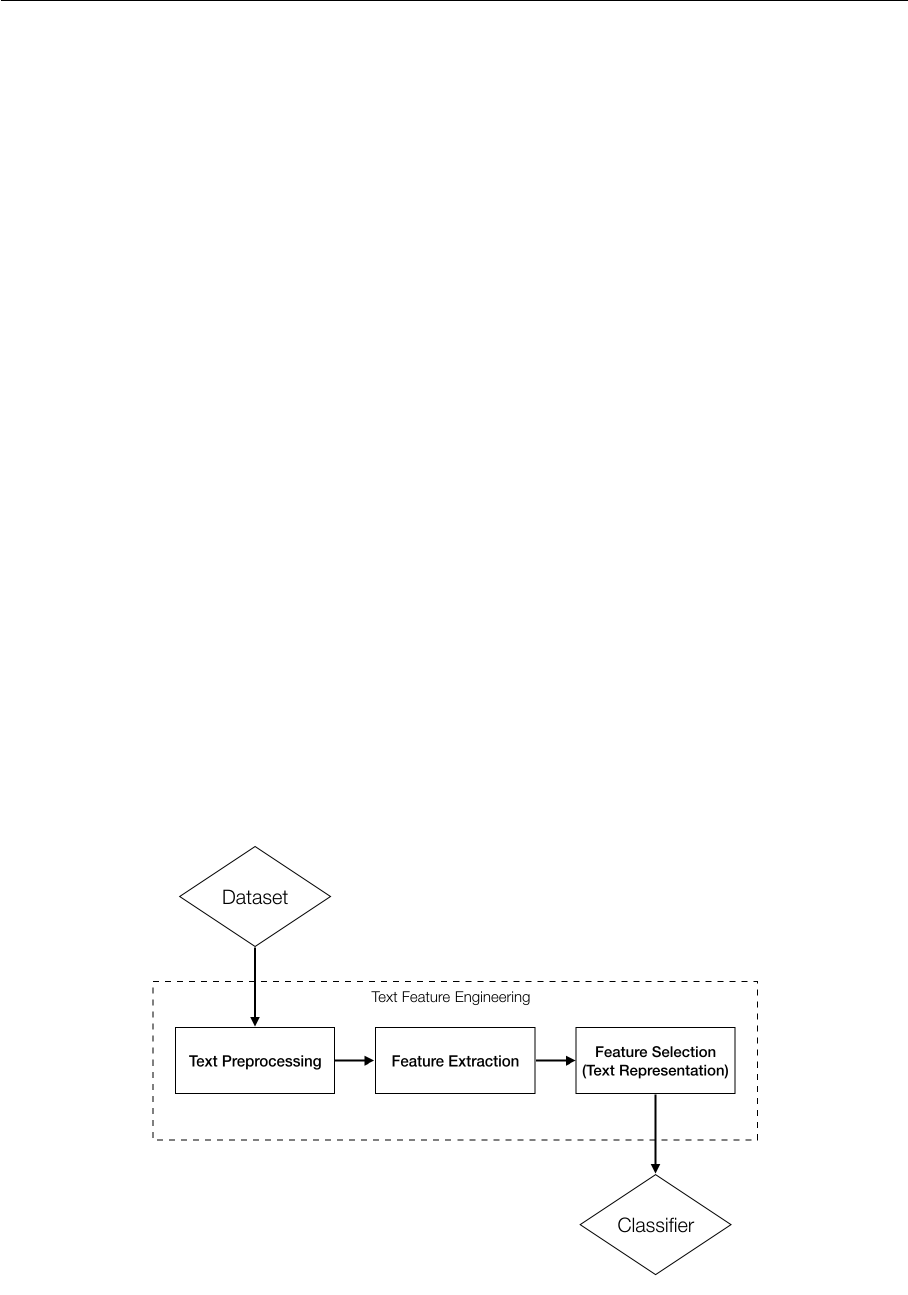
As shown in Figure 2.1, text feature engineering can be divided into three parts: text
preprocessing, feature extraction and feature selection.
Figure 2.1: Text Classification Process
2 BACKGROUND 5
Text preprocessing
Most text data in their raw format aren not well structured and contain lots of unne-
cessary information such as misspelled words, stop-words, punctuations and emojis, etc.
Especially, word segmentation is considered to be a quite important first step for Chine-
se NLP tasks, because unlike English and any other Indo-European languages, Chinese
words can be composed of multiple characters with no spaces appearing between them.
Text preprocessing involves a variety of techniques to convert raw text data into cleaned
and standardized sequences, which can further improve the performance of classifiers. De-
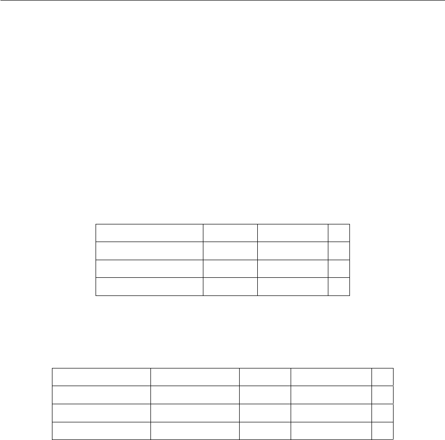
tailed preprocessing methods will be discussed in our experiments. Table 1 and 2 are two
Chinese to English translations with different word segmentation methods.
中外 科学 名著
chinese and foreign scientific masterpiece 4
中 外科学 名著
mid surgery masterpiece 8
Table 1: Chinese to English translation of 中外科学名著 with different word segmentation
methods
北京 大学生 前来 应聘
Peking undergraduates come to apply for jobs 4
北京大学 生前 来 应聘
Peking university while living come to apply for jobs 8
Table 2: Chinese to English translation of 北 京大学生 前来应聘 with different word
segmentation methods
Feature extraction and text representation
The purpose of text representation is to convert preprocessed texts into a form which
computer can process. It’s the most important part which determines the quality of text
classification. Traditional feature extraction techniques include syntactic word represen-
tations such as n-gram, weighted words such as bag-of-words (BoW), and semantic word
representations (word embeddings) such as word2vec, GloVe, etc. Note that vector space
model (VSM)[49] refers to the data structure for each document and BoW refers to what
kind of information we can extract from a document. They are different aspects of cha-
racterizing texts.
BoW is a simple but powerful model to represent text documents. What we need is
just to convert text documents into vectors. Only the uni-gram words are extracted, no

2 BACKGROUND 6
syntax, no semantics and no word position information. Each document is converted into
a vector which represents the frequency of all distinct words that present in the document
vector space.
Here are two simple text documents:
(1) I don’t like this type of movie, but I like this one.
(2) I like this kind of movie, but I don’t like this one.
The uni-grams of these two text documents are:
I, don’t, like, this, type, of, movie, but, I, like, this, one
I, like, this, kind, of, movie, but, I, don’t, like, this, one
Each bag-of-words can be represented as:
BoW1 = {I:2, don’t:1, like:2, this:2, type:1, of:1, movie:1, but:1, one:1}
BoW2 = {I:2, like:2, this:2, kind:1, of:1, movie:1, but:1, don’t:1, one:1}
The document vector space is:
{I, don’t, like, this, type, of, movie, but, one, kind}
The corresponding document vectors are:
[2, 1, 2, 2, 1, 1, 1, 1, 1, 0]
[2, 1, 2, 2, 0, 1, 1, 1, 1, 1]
The biggest shortcoming of this representation is that it ignores text contexts. Every
word is independent of each other and thus can not represent the semantic information
of texts. We can find that these two document vectors are extremely similar in the above
example, which demonstrates that the two sentences have very likely the same meaning.
However they mean the exact opposite. In general, the lexicon in real world applications
is at least one million in size, so BoW model has two serious problems: high dimension
and high sparsity. BoW is the basis of vector space model, so in vector space model we
can reduce the dimension by using feature selection methods and increase the density by
calculating feature weighting factors.
Some algorithms are used to reduce dimensionality, such as principal component ana-

2 BACKGROUND 7
lysis (PCA), independent component analysis (ICA), linear discriminant analysis (LDA),
and latent semantic analysis (LSA), etc. The textual representations using these machine
learning methods are generally considered to be deep representations of the documents.
In addition, distributed semantic word representations are seen as the foundation of deep
learning methods.
Feature selection
When doing the task of text categorization, it is often necessary to extract features from
the documents. Normally we train the model using part of the features which are useful
for learning, rather than using all the features which will eventually lead to curse of di-
mensionality[8] problems.
The feature selection process includes the selection of extracted features and the cal-
culation of feature weights.
The basic idea of feature selection is to rank the original features independently according
to an evaluation metric, we then select some features with the highest score, and filter
out the remaining features. Commonly used supervised feature selection methods include
Relief, Fisher score and Information Gain[35] based methods, etc.[16] Note that feature
selection methods should be distinguished from feature extraction techniques. Feature
extraction is that we create new features from the original datasets, whereas feature se-
lection returns a subset of the initial features. Feature weight calculation mainly refers
to the classic statistical method, term frequency–inverse document frequency (TF-IDF)
method and its extensions.
2.3 Text Classification (Classifiers)
Discriminative methods which directly estimate a decision boundary, such as logistic re-
gression and support vector machine (SVM), generative models which build a generative
statistical model such as naïve bayes, and instance based classifiers which use observations
directly, such as k-nearest neighbor (K-NN), are more traditional but still commonly used
machine learning classification approaches. Tree-based classification algorithms, such as
decision tree and random forests are fast and accurate for text classification.
Deep learning has a significant influence in the fields of image processing, speech recogni-
tion, and NLP. The influence of deep learning on NLP and especially on text classification
is mainly reflected in the following aspects.

2 BACKGROUND 8
End-end training
In the past, when doing statistical natural language processing, experts need to define
various features and need a lot of domain knowledge. Sometimes it is not easy to find
a good feature. But with end-to-end training, as long as there are pairs of inputs and
outputs (input-output), what we need to do is just labeling the output corresponding to
the input in order to form a training data set. The learning system can be then esta-
blished through automatic training using neural networks, without artificial settings and
carefully designed features. This has changed the development of many NLP technologies
and greatly reduced the technical difficulties of NLP. This means that as long as we have
enough computational resources (GPU, TPU) and labeled data, we can basically imple-
ment the NLP model and get really good results, which promotes the popularity of NLP
technologies.
Semantic representation (word embeddings)
One of the commonly used semantic representations is context-free embedding, which
means that the representation of a word is fixed (represented by a multi-dimensional vec-
tor) regardless of its context. The other representation depends on the context of different
sentences, the meaning of the same word might be different, so its embeddings are also
accordingly different. Now using models like BERT and GPT, we can train and obtain
the dynamic embedding of a word based on its context.
Pre-trained model
We know that neural networks need to be trained with data, they extract information from
data and convert them into corresponding weights. These weights can be then extracted
and transfered to other neural networks. Because we’ve transfered these learned features,
when we try to solve a similar problem, we don’t need to train a new neural network
model from scratch, instead we can start with models that have been trained to solve
similar problems. By using pre-trained models which are previously trained with massive
amounts of data, we can apply the corresponding structures and weights directly to the
problems we are facing. This process is called Transfer Learning. Since the pre-trained
models have been well trained, we don’t need to modify too many weights, what we need
to do is just modifying some parameters. And this is called Fine Tuning. As a result, the
pre-trained model can significantly reduce the training time.
Sentence encoding methods (CNN/RNN/LSTM/GRU/Transformer)
For a sentence of variable length, it can be encoded with RNN, LSTM, GRU or Transfor-
mer. Although these several encoding methods for sentences are feasible, recently we tend
to use Transformer to encode sentences. We can apply the encoded sentences in various

2 BACKGROUND 9
NLP applications such as machine translation, question answering, language modeling,
sentiment analysis, text classification and so on.
Attention
Encoder-Decoder model[52], or sequence to sequence (seq2seq) model, was first introdu-
ced in 2014 by Google. In an Encoder-Decoder neural network, a set of RNNs / LSTMs /
GRUs encode an input sequence into a fixed-length internal representation, another set of
RNNs / LSTMs / GRUs read this internal representation and decodes it into an output se-
quence. The length of the input and output sequences might differ. This Encoder-Decoder
architecture has achieved excellent results on a wide range of NLP tasks, such as question
answering and machine translation. Nevertheless, this approach suffers from the problem
that neural networks are forced to compress all the necessary information of an input
sequence into a fixed-length internal vector, which makes it difficult for neural networks
to deal with longer sequences, especially those in the test set which are longer than the
sequences in the training set.[7] First, the internal semantic vector cannot fully represent
the information of the entire input sequence. Second, the pre-existent information will be
overwritten by the newly input messages.
The attention mechanism is a way to free the Encoder-Decoder structure from fixed-length
internal representations. It maintains the encoder’s intermediate outputs from each step
of the input sequences, and then trains the model to learn how to selectively focus on the
inputs and relate them to the items in the output sequences. In other words, each item
in the output sequence depends on the selected item in the input sequence.[1]
Although this mechanism increases the model’s computational complexity, it is able to
result in a better performance, even state-of-the-art. Additionally, the model can also
show how to pay attention to input sequences when predicting output sequences. Un-
like the situation in computer vision, where several approaches for understanding and
visualizing CNNs have been developed, it’s normally pretty hard to visualize and under-
stand what neural networks in NLP have learned.[5] Thus this mechanism helps us to
understand and analyze what the model is focusing on and how much it focuses on a
particular input-output pair. Further attention visualization examples can be found in
machine translation[7], text summarization[48], speech recognition[13] and image descrip-
tions[56], etc.

3 RELATED WORK 11
3 Related Work
A central study in text classification is feature representation, which is commonly based
on the bag-of-words (BoW) model. Besides, feature selection methods, such as TF-IDF
model, LSA, sLDA, are applied to select more discriminative features. The major classi-
fiers in the traditional machine learning era are mainly based on naïve bayes, maximum
entropy, k-nearest neighbor (K-NN), decision tree and support-vector machine (SVM).
Traditional machine learning algorithms for text classification are well summarized in
[6][29].
3.1 Text Classification
Text categorization escapes the process of artificial feature design, text similarity com-
parison and distance definitions in the era of deep learning, but still can not escape the
choice of text preprocessing, feature extraction, model selection, parameter optimization,
coding considerations (one-hot, n-gram, etc.) and time cost trade-off.
In summary, there are six main types of deep learning models:
(1) Vector representation of words: word2vec, GloVe, FastText, BERT, GPT, ELMo,
etc.
(2) Convolutional neural network feature extraction: TextCNN, CharCNN, DCNN, VD-
CNN, etc.
(3) Pre-training & multi-task learning: BERT, GPT, ELMo, etc.
(4) Context mechanism: TextRNN, BiRNN, RCNN, etc.
(5) Memory storage mechanism: EntNet, DMN, etc.
(6) Attention mechanism: HAN, etc.
In the following paragraph we will get into a little details of the above models and get a
global picture of the application and development of deep learning in text classification
in recent years.
3.1.1 Vector Representation of Words
FastText[25], which is not much innovative in academics but has very outstanding perfor-
mance, was proposed by Mikolov’s team in Facebook in 2016. FastText (shallow network)
3 RELATED WORK 12
can often achieve the accuracy comparable to deep network in text classification, but is
many orders of magnitude faster than deep network in training time. The core idea of
FastText is to superimpose the word and n-gram vectors of the whole document to obtain
a document vector, then we use this document vector to do softmax multiclassificati-
on. There are two techniques involved: character-level n-gram features and hierarchical
softmax classification. Hierarchical softmax is first introduced in word2vec which we will
discuss in the next chapter, so here we only focus on character-level n-gram.
Word2vec treats each word in the corpus as atomic. For each word it generates a vec-
tor, which ignores the words’ internal morphological features. For example, “country” and
“countries”, these two words have many characters in common, in other words, they have
similar internal forms. However, in traditional word2vec model, such words lose this in-
ternal information when converted to different IDs. To overcome this problem, FastText
uses character-level n-grams to represent a word. For word “country”, assuming that the
value of n is 3, then its trigram are as follows:
<co, cou, oun, unt, ntr, try, ry>
where < indicates a prefix and > indicates a suffix. So we can use these trigrams to
represent word “country”. Furthermore, we can stack and add up the vector of these seven
trigrams to represent word “country”.
This brings two benefits: First, it will generate better word vectors for low frequen-
cy words, because their n-grams can be shared with other words. Second, for out-of-
vocabulary (OOV) words, we can still produce their word vectors by superimposing their
character-level n-gram vectors. Whereas in word2vec OOV words are either zero or ran-
domly initialized.
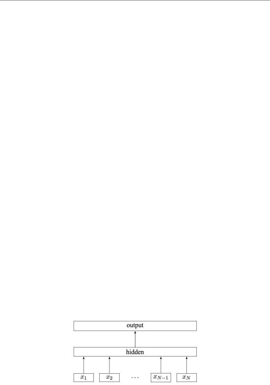
Figure 3.1: Model architecture of FastText for a sentence with N ngram features
x
1
, ..., x
N
. The features are embedded and averaged to form the hidden variable.
3 RELATED WORK 13
As we can see in Figure 3.1, like Continuous Bag of Words (CBOW), FastText has three
layers: input layer, hidden layer and output layer (hierarchical softmax). They have so-
mething in common. Their input are words represented by multiple vectors; they have a
specific target value; the hidden layers are averages of multiple superimposed word vec-
tors. The difference is that the input of CBOW is the context of the target word whereas
the input of FastText is multiple words and their character-level n-gram features, which
are used to represent a single document; the input words of CBOW are one-hot vectors
whereas the input of FastText are embedded vectors; the output of CBOW is the target
word where the output of FastText is the class label corresponding to the document.
In a word, FastText is a pretty simple but violent classification model. For paragraph
reasons, global vectors for word representation (GloVe) will not be discussed here.
3.1.2 Convolutional Neural Network Feature Extraction
TextCNN[28], which has become a classical deep learning model in text categorization,
was proposed by Kim in 2014.
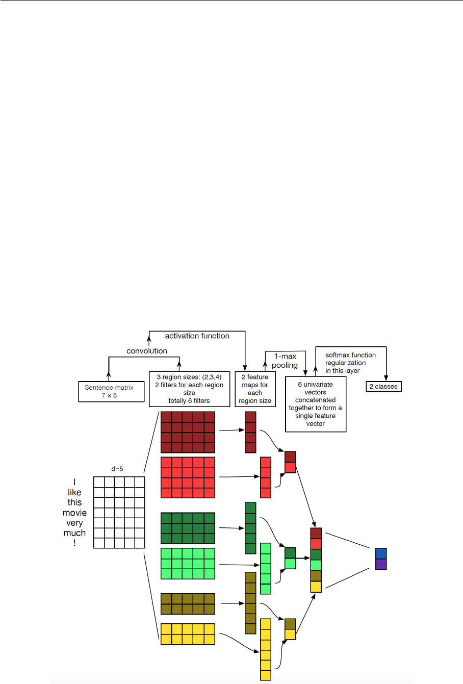
Figure 3.2: CNN architecture for sentence classification (adopted from Zhang 2014 [63])

3 RELATED WORK 14
As shown in Figure 3.2, the input layer is a 7 × 5 matrix. 5 is the word vector dimension
and the sentence length is 7. The second layer uses 3 sets of convolution kernels with
width of 2, 3 and 4, each size has 2 kernels. Each of the convolution kernels slides over
the whole sentence to generate a feature map. In the figure, the kernel does not use pad-
ding during the sliding process. The convolution kernel with width of 4 slides over the
sentence of length 7, we can get a feature map of length 4. 1-max pooling is performed
over each map. Thus a univariate feature vector is generated from all the 6 maps, and
these 6 features are concatenated to form one final feature vector. The final output layer
receives this feature vector as input and uses it to classify the sentence.
Over the last several years deep learning methods especially convolutional neural networks
(CNN) have been shown to outperform previous state-of-the-art machine learning techni-
ques in computer vision. But when CNN is first used in NLP, we’re faced with different
problems.
The max pooling operation in CNN has advantages: it has feature’s position and rotation
invariant characteristics, because no matter where the feature appears in a sentence, it
can be extracted regardless of its position. Besides, max pooling can reduce the number of
model parameters, which is beneficial to reduce the model over-fitting problem. However
in NLP this advantage isn’t necessarily a good thing, because in many NLP applications
the location information of the features is very important, for example, negative words
appear in different positions, resulting in completely different sentence meanings:
I don’t like this type of movie, but I like this one.
I like this kind of movie, but I don’t like this one.
So for TextCNN the completely loss of feature’s location information is its Achilles’ heel.
In summary, in TextCNN convolution is used to extract key information similar to n-
grams. We are able to capture features between multiple consecutive words and share
weights and biases when calculating the same type of features.
The overall performance of TextCNN is good, but there are problems. The local receptive
field size (filter size) is fixed, it is difficult to determine the filter size. The ability to mo-
del longer sequence is limited. Most importantly, the feature’s location information is lost.
Based on CNN, some models are proposed recently. Especially, due to the above pro-
blems, several works have been done.
Kalchbrenner and Blunsom et al. (2014)[27] introduced dynamic convolutional neural

3 RELATED WORK 15
network (DCNN). It uses dynamic k-max pooling, where the result of pooling isn’t a
maximum value, but the k-maximum values, which is a subsequence of the original in-
put. This brings several benefits. The dynamic k-max pooling better preserves multiple
important information in a sentence. The number of extracted features varies according
to the length of the sentence. Besides, it preserves the relative positions between words
and the word position information. It also takes into account the semantic information
between words which are far away in a sentence.
Zhang et al. (2015)[63] conducted a variety of very good comparative experiments on
CNN models mentioned in [28], and provide us with some CNN architecture and hyper-
parameter setting advice.
Zhang and LeCun (2015)[62] proposed character-level convolutional neural network (Char-
CNN) which is also an effective model. The most important point of their experimental
conclusion is that this model can classify text without using words, which strongly sug-
gests that the human language can also be considered as a signal that is no different from
any other type of signals.
Conneau and Lecun et al. (2016)[14] first used very deep convolutional neural network
(VDCNN) in NLP. Prior to their work, normally very shallow CNNs are used in text
categorization. In their work they utilize 29 convolution layers to improve the accuracy of
text classification. They get some important discoveries by exploring deep architectural
approaches: VDCNN performs better on big datasets; deeper network depth can improve
the model performance; etc.
Zhang and LeCun (2017)[61] did an interesting experiment which shows that FastText
model has better results in character-level encoding for Chinese, Japanese, and Korean
texts (CJK language), and better results in word-level encoding for English texts.
3.1.3 Pre-training & Multi-task Learning
Pre-training is a conventional method in computer vision since deep learning has become
popular. We already know that for hierarchical CNN structure, neurons of different layers
can learn different types of image features. For example, if we have a face recognition
task, after having trained the network, we visualize the features learned by each layer of
neurons, we will see that the lowest hidden layer of neurons learn has learned features
such as colors and lines, the second layer facial organ, and the third layer facial contour.
The lower the layer, the more basic the features. The upper the layer, the more related to
the task the extracted features. Because of this, the pre-trained network parameters, espe-

3 RELATED WORK 16
cially the features extracted from the bottom layers, are more independent of the specific
task, and more general. This is why we normally initialize new models with pre-trained
parameters of bottom layers.
What about NLP? The general choice for pre-training in NLP is to use language mo-
dels. The neural probabilistic language model introduced by Bengio et al. (2003)[9] can
not only predict the next word given the last few words, but also obtain a by-product, a
matrix, which is actually the word embedding matrix. Ten years later, the word2vec mo-
del proposed by Mikolov et al. (2013)[40], which simply aims to obtain word embeddings,
has become more and more popular.
So what is pre-training in NLP? Given a NLP task, such as text classification or question
answering, each word in a sentence is one-hot encoded as input, then multiplied by the
learned word embedding matrix, so we get the words’ corresponding embeddings. This
seems to be a looking-up operation, but in fact, the word embedding matrix is actually
the network parameter matrix which maps the one-hot layer to the embedding layer. So in
other words, the network from one-hot layer to embedding layer is equivalently initialized
with this pre-trained embedding matrix.
However the most serious problem with previous word embedding models is they can
not deal with polysemy. We know that polysemy is a phenomenon that often occurs in
human languages. What’s the negative impact of polysemous words on word embeddings?
For example:
He jumped in and swam to the opposite bank.
My salary is paid directly into my bank.
As shown above, “bank” has two meanings, but when we encode this word, the word
embedding model can’t distinguish between these two meanings. Despite the fact that
the contextual words of these two sentences are different, when the model being trained,
it will always predict the same word “bank”. The same word “bank” occupies the same
word embedding space (the same line in the matrix) of the model, which causes two
different context information encoded into the same parameter space. As a result, word
embeddings can’t distinguish the different semantics of polysemous words.
Researchers have made an astonishing and huge progress in NLP in 2018. Large-scale
pre-trained language models like OpenAI GPT and BERT perform quite well on various
NLP tasks using generic model architectures. The idea is similar to pre-training in com-
puter vision that we have discussed previously. But even better than that, the newly

3 RELATED WORK 17
proposed approaches do not require labeled data for pre-training. They make use of unla-
beled data, which is obviously inexhaustible in real world, allowing us to extract a large
amount of linguistic knowledge and encode them into the models. Integrating linguistic
knowledge as much as possible will naturally enhance the generalization ability of the mo-
dels, especially when we have limited amount of data. And introducing priori linguistic
knowledge has always been one of the main purposes of NLP, especially in deep learning
scenarios.
Deep contextualized word representations (ELMo) proposed by Peters et al. (2018)[44]
dynamically adjust word embedding based on current context. The core idea of ELMo
is that, we first learn word embeddings after we have trained language model, at this
time the polysemous words still can not be distinguished. But when we actually use word
embeddings, the words already have a specific context. Then we can adjust the word em-
bedding according to the semantics of the word. The adjusted word embedding can better
express the specific meaning in its context, which cleverly solve the problem of polysemy.
ELMo has a typical two-phase process. The first step is the use of language models for
pre-training, called feature-based pre-training. The second step is to extract the word
embedding of the corresponding word in each layer of the pre-trained model. Each word
in a sentence can get three embeddings: in the bottom layer we get word embedding; the
embedding in the first layer of long short-term memory (LSTM) captures word’s syntac-
tic information; the embedding in the second layer of LSTM captures word’s semantic
information. We then combine the extracted embeddings together as a new feature in the
downstream NLP tasks. ELMo can improve its performance in 6 different NLP tasks.
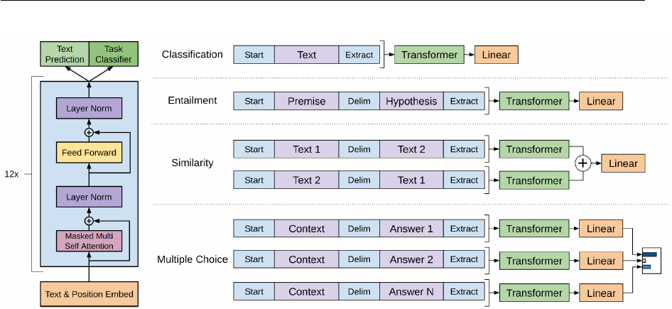
Generative pre-training model (OpenAI GPT) introduced by Radford et al. (2018)[45] al-
so has a two-phase training process, see Figure 3.3. In the first phase we use the language
model for pre-training and in the second phase we fine-tune the model to solve downstream
tasks. Despite of the similarity between GPT and ELMo, GPT has two major differences
from ELMo. The first difference is that in GPT’s second step, we need to fine-tune the
same base model so that we can use it in the following downstream tasks. We also need
substantial task-specific architecture modifications. The second difference between GPT
and ELMo is that GPT uses Transformer as its feature extractor. Transformer, introduced
by Vaswani et al. (2017)[54], which is first used in neural machine translation (NMT), is
a novel neural network architecture based on a self-attention mechanism. Why do we use
Transformer here? Because Transformer is currently the best feature extractor. Transfor-
mer outperforms recurrent neural network (RNN) because RNN can not be parallelized.
Transformer also outperforms CNN because it can capture long-distance features. Ad-
ditionally, in the pre-training step of GPT, although we still use the language model as
3 RELATED WORK 18
Figure 3.3: (left) Transformer architecture and training objectives used in GPT. (right)
Input transformations for fine-tuning on different tasks. We convert all structured in-
puts into token sequences to be processed by the pre-trained model, followed by a line-
ar+softmax layer. (adopted from [45])
target task, we adopt a single-direction language model. That is, one limitation with GPT
is that it is only trained to predict the future left-to-right context, without right-to-left
context. The result of GPT is very amazing. It achieves the best results in 9 out of 12
NLP tasks.
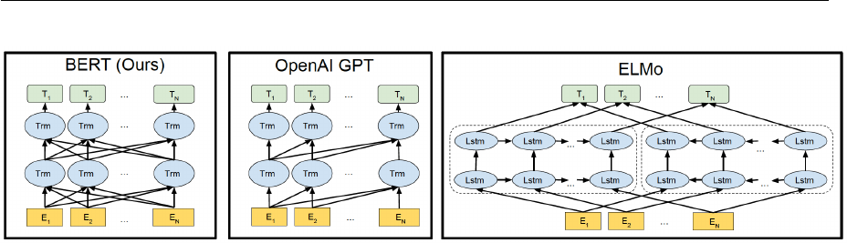
Now we finally come to the new language representation model, deep bidirectional en-
coder representations from transformers (BERT), proposed by Devlin et al. (2018)[18],
which obtains new state-of-the-art results in 11 NLP tasks including text classification.
BERT has the same two-phase process as GPT. It is designed to pre-train deep bidirec-
tional representations by jointly conditioning on both left and right context in all layers.
The pre-trained BERT representations can be fine-tuned with just one additional output
layer. They also proposed masked language model and next-sentence prediction method
in order to pre-train the model in both forward and backward directions. BERT input
representations are the sum of the token embeddings, the segmentation embeddings and
the position embeddings.
There is a close relationship between the above 3 models, see Figure 3.4. If we change
GPT model in the pre-training phase by using bidirectional language model, then we will
get BERT. If we replace ELMo’s feature extractor LSTM with Transformer, we will also
get BERT.
In summary, inductive transfer learning consists of two steps: pre-training, in which the
3 RELATED WORK 19
Figure 3.4: Differences in pre-training model architectures. BERT uses a bidirectional Trans-
former. OpenAI GPT uses a left-to-right Transformer. ELMo uses the concatenation of inde-
pendently trained left-to-right and right-to-left LSTM to generate features for downstream
tasks. Among three, only BERT representations are jointly conditioned on both left and
right context in all layers. (adopted from [18])
model learns a general-purpose representation of inputs by using a specific feature extrac-
tor (RNN, LSTM, Transformer), and adaptation, in which the representation is transferred
to a new task.[43] As we discussed previously, there are two main paradigms for adap-
tation: feature ensemble (ELMo) and fine-tuning (GPT, BERT). For ELMo, we extract
contextual representations of the words from all layers by feeding the input sentence into
pre-trained bidirectional LSTM network. During adaptation, we learn a linear weighted
combination of word embeddings in all layers which is then used as input to a task-specific
architecture in downstream tasks. In contrast, for GPT and BERT, after obtaining the
pre-trained model, during fine-tuning (adaption), we still adopt the same model, use part
of the training data of the downstream task, train on the same model to correct the
network parameters obtained during the pre-training stage. We only need a task-specific
output layer. So which paradigm is better? Peter et al. (2019)[43] did some research to
empirically compare feature ensemble with fine-tuning approaches across diverse datasets.
They come to a conclusion that the relative performance of two approaches depends on
the similarity of the pre-training and target tasks. So for BERT, we would better fine-tune
the model.
3.1.4 Context Mechanism
We know that the nature of convolution is to extract features. Deep learning is about
feature representation learning. But documents or sentences are sequences, that is, the
previous input is related to the subsequent input. So thinking about to use RNN to deal
with texts seems to be reasonable. Recurrent neural network for text classification (Tex-
tRNN) proposed by Liu et al. (2016)[37], whose architecture is similar to TextCNN, is the
first RNN model to classify documents. RNN and its variants can capture variable-length
and bidirectional n-gram information. But it has disadvantages. As far as I’m concerned,

3 RELATED WORK 20
this model is not recommended because the training speed of RNN is very slow. RNN is
also a biased model, in which later words are more dominant than earlier words.
Recurrent convolutional neural network (RCNN) which was introduced by Lai et al.
(2016)[33] is a combination of CNN and RNN. They employ a bidirectional RNN to
capture the contexts and learn the word representations. They also employ max-pooling
to automatically determine which feature plays a more important role in text classificati-
on. This model runs faster than RNN and gets a good result in three of the four commonly
used datasets.
3.1.5 Memory Storage Mechanism
Typical Encoder-Decoder model’s performance is limited by the size of its memory, espe-
cially when dealing with longer sequences. This limitation can be solved by a strategy
called attention mechanism which was proposed by Bahdanau et al. (2014)[7]. We can
also refine the attention mechanism by adding a separate, readable and writable memo-
ry component. Dynamic memory networks (DMN) which was proposed by Kumar et al.
(2016)[32] has four modules: input module, question module, episodic memory module
and answer module. Here the input is a list of sentences, the question module is equiva-
lent to the gated units which uses the attention mechanism to selectively store the input
information in the episodic memory module. Then the output of episodic memory is ans-
wered by the answer module. The DMN obtains state-of-the-art results on several types
of tasks and datasets including text classification.
3.1.6 Attention Mechanism
Hierarchical attention network (HAN) proposed by Yang et al. (2016)[59] is another model
in which attention mechanism is introduced. The basic idea of HAN is that we first con-
sider the hierarchical structure of documents: a sentence is a group of words, a document
consists of several sentences. So we can divide documents hierarchy into three layers, that
is: words, sentences and texts. We use two bidirectional LSTMs to model word-sentence
and sentence-document. Second, different words and sentences contain different informa-
tion thus they can not be treated equally. The attention mechanism is introduced in each
model to capture longer dependencies. From this we derive the importance of different
words and sentences when constructing sentences and texts accordingly.
The HAN model structure is very consistent with the human understanding process:
word → sentence → document. The most important thing is that the attention layers
can be well visualized when providing us with better classification accuracy. At the same

3 RELATED WORK 21
time, we can find that the attention part has a great influence on the expression ability
of the model.
3.2 Short Text Classification
Traditional machine learning methods for short text classification are mainly based on
widely used machine learning models, such as SVM, etc. Next we focus on deep learnings
methods for short text classification which has dominated in research in recent years.
Wang et al. (2017)[55] introduced knowledge from a knowledge base and combine words
with associated concepts to enrich text features. They also use character level information
to enhance word embeddings. They finally build a joint CNN model to classify short texts.
Our work is similar to their work, the difference is that we enrich word embeddings with
entities while they utilize concepts. We also adopt the same datasets they used in the
experiments.
Zeng et al. (2018)[60] proposed topic memory networks which jointly explore latent topics
and classify documents in an end-to-end system.
3.3 Text Classification using Named Entities
There is not much research work about text classification using named entities. Kral
(2014)[30] compared five different approaches to integrate named entities using naïve
bayes classifier on Czech corpus in his work. The experimental results show that entity
features do not significantly improve the classification performance over the baseline word-
based features. The improvement is maximum 0.42%.

4 WIKIPEDIA2VEC AND DOC2VEC 23
4 Wikipedia2Vec and Doc2Vec
One of our main concerns is to get good entity vectors. Our entity vectors are generated
by using Wikipedia2Vec and Doc2Vec. Wikipedia2Vec, which is implemented by Yamada
et al. (2018)[57], is an open source tool used for obtaining vector representations of words
and entities from large corpus Wikipedia. This tool enables us to learn both the vectors of
words and entities simultaneously and thus places similar words and entities close to each
other in a high dimensional continuous vector space. Compared with existing embedding
tools such as Gensim[46], FastText[25] and RDF2Vec[47], this tool has been proved to be
the state-of-the-art NLP model in the named entity disambiguation (NED) task.
4.1 Word2vec and Skip-gram
The word2vec model, which was proposed by Mikolov et al. (2013)[40], has caught rese-
archers a numerous amount of attention in recent years. The core idea of word2vec is to
characterize one word through the neighbors of this word with prediction between every
word and its context words. The word vector representations produced by the model have
been proven to carry semantic features and can be subsequently used in many natural
language processing applications and further research.
Word2vec actually contains two algorithms, that is, skip-gram, which predicts context
words given target; continuous bag of words (CBOW), which predicts target word from
bag-of-words context. The model also contains two moderately efficient training methods,
hierarchical softmax and negative sampling[39].
Figure 4.1: Word based skip-gram model
We now focus on skip-gram algorithm. Given a sentence of T words w
1
, w
2
, ..., w
T
, for
each word t = 1 . . . T , we predict surrounding words in a window of “radius” m of every
word. Here m is the size of the context window, w
t
denotes the center word and w
t+j
is its

4 WIKIPEDIA2VEC AND DOC2VEC 24
context word. The objective function is to maximize the probability of any context word
given the current center word. We want to maximize the following objective function:
J
0
(θ) =
T
Y
t=1
Y
−m≤j≤m
j6=0
P (w
t+j
|w
t
; θ) (4.1)
Machine learning likes minimizing things so we add minus. T represents the normalization
per word, so the objective function does not depend on the length of the sentence.
J(θ) = −
1
T
T
X
t=1
X
−m≤j≤m
j6=0
log P (w
t+j
|w
t
) (4.2)
So we minimize the negative log probability where θ represents all variables we will opti-
mize.
For the conditional probability P (w
t+j
|w
t
), the simplest formulation is:
P (o|c) =
exp(u
T
o
v
c
)
P
V
w=1
exp(u
T
w
v
c
)
(4.3)
where o is the outside (or output) word index, c is the center word index, v
c
and u
o
are
“center” and “outside” vectors of indices c and o, V is a set containing all the words in the
vocabulary. Note we have two vectors for each word because it makes math much easier.
This softmax function uses word c to obtain probability of word o. We use softmax func-
tion because it’s sort of a standard way to turn numbers into a probability distribution.
We now compute derivatives of equation 4.3 to work out minimum.
∂
∂v
c
log
exp(u
T
o
v
c
)
P
V
w=1
exp(u
T
w
v
c
)
=
∂
∂v
c
log exp(u
T
o
v
c
) −
∂
∂v
c
log
V
X
w=1
exp(u
T
w
v
c
) (4.4)
For the left part of the formula, we have
∂
∂v
c
log exp(u
T
o
v
c
) =
∂
∂v
c
(u
T
o
v
c
) = u
o
(4.5)
For the right part of the formula, by using chain rule we have

4 WIKIPEDIA2VEC AND DOC2VEC 25
∂
∂v
c
log
V
X
w=1
exp(u
T
w
v
c
) =
1
P
V
w=1
exp(u
T
w
v
c
)
·
∂
∂v
c
V
X
x=1
exp(u
T
x
v
c
)
=
1
P
V
w=1
exp(u
T
w
v
c
)
·
V
X
x=1
∂
∂v
c
exp(u
T
x
v
c
)
!
=
1
P
V
w=1
exp(u
T
w
v
c
)
·
V
X
x=1
exp(u
T
x
v
c
)
∂
∂v
c
(u
T
x
v
c
)
!
=
1
P
V
w=1
exp(u
T
w
v
c
)
·
V
X
x=1
exp(u
T
x
v
c
)u
x
!
(4.6)
Combining formula 4.5 with 4.6 we get the final derivative of conditional probability
P (w
t+j
|w
t
), that is
∂
∂v
c
log(P (o|c)) = u
o
−
1
P
V
w=1
exp(u
T
w
v
c
)
·
V
X
x=1
exp(u
T
x
v
c
)u
x
!
= u
o
−
V
X
x=1
exp(u
T
x
v
c
)
P
V
w=1
exp(u
T
w
v
c
)
· u
x
= u
o
−
V
X
x=1
P (x|c) · u
x
(4.7)
Besides, we can observe that the minuend in formula 4.7 is an expectation, which is an
average over all the context vectors weighted by their probability. The above formula is
just the partial derivatives for the center word vector parameters. Similarly, we also need
to compute the partial derivatives for the output word vector parameters. Finally, we have
derivatives with respect to all the parameters and we can minimize the cost(loss) function
using gradient descent algorithm.
4.2 Wikipedia2Vec
Wikipedia2Vec iterates over the entire Wikipedia pages. It extends the conventional word
vector model (i.e., skip-gram model) by using two submodels: Wikipedia link graph model
and anchor context model. It then jointly optimizes these three models.
4.2.1 Wikipedia Link Graph Model
Wikipedia link graph model[58] is a model which learns entity vectors by predicting neigh-
boring entities in Wikipedia’s link graph. Wikipedia’s link graph is an undirected graph
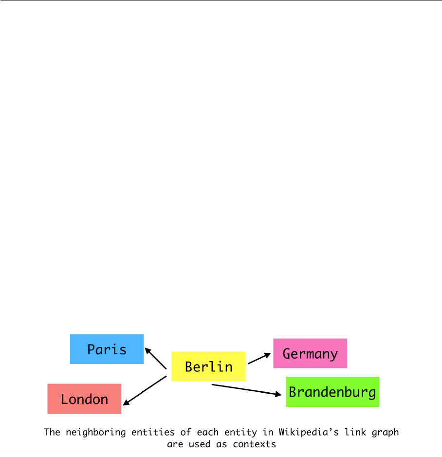
4 WIKIPEDIA2VEC AND DOC2VEC 26
whose nodes represent entities and edges represent links between entities in Wikipedia.
Entity linking (EL) is the task of recognizing (named entity recognition NER) and lin-
king (named entity disambiguation NED) a named-entity mention to an instance in a
knowledge base (KB), typically Wikipedia-derived resources like Wikipedia, DBpedia and
YAGO.[12]
NED in NLP is a task to determine the identity of entities which are mentioned in do-
cuments. For example, given the sentence “Washington is the capital city of the United
States”, here we aim to determine that Washington refers to “Washington, D.C.” and not
to “George Washington”, the first President of the United States. EL requires a KB that
contains entities. Wikipedia2Vec is obviously based on Wikipedia, in which each page is
regarded as a named entity. For example the page of Washington, D.C. in Wikipedia has
a link to the page of United States, so there is an edge between this pair of entities. There
are also some other cases, for example, Berlin has a link to Germany, Germany has a link
to Berlin, both of the entities are linked to each other.
Figure 4.2: Wikipedia link graph model
Given a set of entities e
1
, e
2
, ..., e
n
, for each entity e
i
, we compute the probability of every
entity in the set that is linked to this entity e
i
. Here E denotes the set of all the entities
in KB and S
e
is the set of entities which has a link to entity e. We want to maximize
the probability of any entity that has a link to entity e given this entity e. So we need to
minimize this following objective function:
J
e
= −
X
e
i
∈E
X
e
o
∈S
e
i
,e
i
6=e
o
log P (e
o
|e
i
) (4.8)
For the conditional probability P (e
o
|e
i
), we compute it using the following softmax func-
tion:

4 WIKIPEDIA2VEC AND DOC2VEC 27
P (e
o
|e
i
) =
exp(u
T
e
o
v
e
i
)
P
e∈E
exp(u
T
e
v
e
i
)
(4.9)
4.2.2 Anchor Context Model
So far we have learned entity vectors using entities and word vectors using words. We
obtain these vectors by training two different models, so the words and entities are map-
ped into different vector spaces. We hope to map them into the same vector space so we
introduce anchor context model[58] which learns entity vectors and word vectors simul-
taneously by predicting the context words given an entity.
In anchor context model, we want to predict the context words of an entity pointed
to with target anchor.[58] Here A denotes the set of anchors in KB. Each anchor in A
contains a referent entity e
i
and a set of its context words S. The previous c and next
c words of a referent entity are seen as its context words. The objective function is as
follows:
J
a
= −
X
(e
i
,S)∈A
X
w
o
∈S
log P (w
o
|e
i
) (4.10)
Figure 4.3: Anchor context model
For the conditional probability P (w
o
|e
i
), we compute it using the following softmax func-
tion:
P (w
o
|e
i
) =
exp(u
T
w
o
v
e
i
)
P
w∈W
exp(u
T
w
v
e
i
)
(4.11)

4 WIKIPEDIA2VEC AND DOC2VEC 28
4.3 Doc2Vec
Doc2Vec is proposed by Quoc Le and Tomas Mikolov in 2014.[34] Doc2Vec, also called
Paragraph Vector, is an unsupervised algorithm, with which we are able to get fixed-
length feature representations from variable-length documents. Doc2Vec can be used on
text classification and sentiment analysis tasks.
Similar to word2vec, Doc2Vec also has two training algorithms, that is, distributed bag
of words (DBOW) which is similar to skip-gram in word2vec, and distributed memory
(DM) which is similar to continuous bag of words (CBOW) in word2vec. Especially, the
input of DBOW is the paragraph vector. The model is trained to predict the words in
a small window. In contrast to DBOW, in DM, the paragraph vector and local context
word vectors are concatenated or averaged to predict the next word in a context.
Quoc Le also did experiments trained on Wikipedia which shows that the Paragraph
Vector algorithms perform significantly better than other methods and embedding quality
is enhanced.[15] So in our work, we train the Doc2Vec model on Wikipedia dump and use
Doc2Vec to obtain better entity embeddings.

5 CONVOLUTIONAL NEURAL NETWORK FOR SHORT TEXT CLASSIFICATION 29
5 Convolutional Neural Network for Short Text Clas-
sification
In this section, we modify traditional convolutional neural network for text classification
(TextCNN) and propose a new model called convolutional neural network with entities for
text classification (EntCNN), using words as well as entities to extract more contextual
information from texts. We first introduce the way to obtain entities and entity vectors
from texts. Then we describe our model to show how to learn features from words and
entities.
5.1 Entity Linking
The first step of our work is to detect named entities from texts. A named entity is, rough-
ly speaking, anything that can be referred to with a proper name: a person, a location or
an organization.[26] As we have mentioned in chapter 4, entity linking (EL) is the task
of recognizing and disambiguating named entities to a knowledge base (KB). It is some-
times also known as named entity recognition and disambiguation. Why can we benefit
from EL? By linking named entity mentions appearing in texts with their corresponding
entities in a KB, we can make use of KB which contains rich information about entities to
better understand documents. EL is essential to many NLP tasks, including information
extraction, information retrieval, content analysis, question answering and knowledge ba-
se population.[50] Shen and Jiawei Han et al. (2014) wrote an outstanding survey about
EL, see [50].
In our work, we utilize TagMe to extract entities and link them to Wikipedia entries.
TagMe is an end-to-end system which has two major stages. First, we process a text to
extract named entities (i.e. named entity recognition). Then we disambiguate the extrac-
ted entities to the correct entry in a given KB (i.e. named entity disambiguation). After
having obtained entity entries in a KB, we use Wikipedia2Vec to get entity vectors. As we
have discussed in the previous chapter, Wikipedia2Vec is a disambiguation-only approach.
In contrast to end-to-end approach, this model takes standard named entities directly as
input and disambiguates them to the correct entries in a given KB. In our work, we just
need to query previously obtained entity entries on Wikipedia2Vec, then we can get entity
vectors as output.
5 CONVOLUTIONAL NEURAL NETWORK FOR SHORT TEXT CLASSIFICATION 30
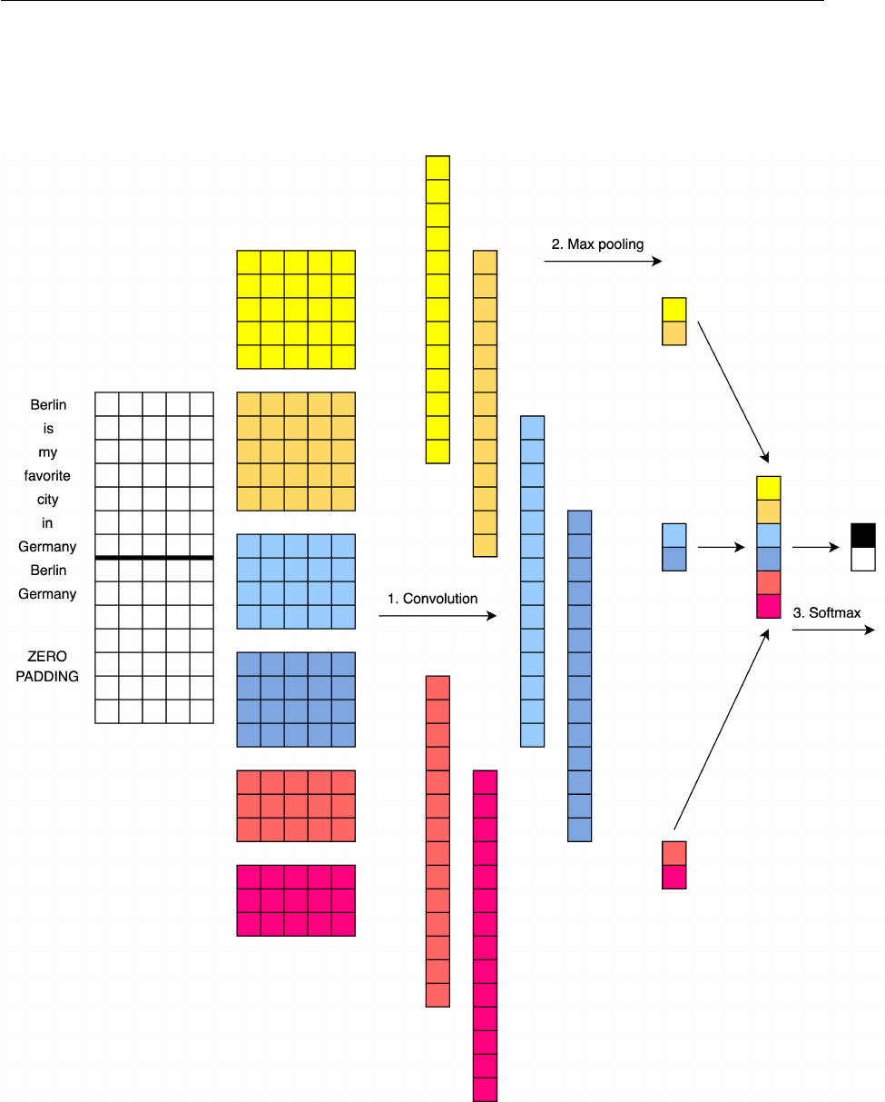
Figure 5.1: Convolutional neural network with words and entities for short text classifi-
cation

5 CONVOLUTIONAL NEURAL NETWORK FOR SHORT TEXT CLASSIFICATION 31
5.2 Overall Architecture of EntCNN
As we have discussed in chapter 3, CNNs have achieved impressive results on text classi-
fication tasks. In our work, we focus on single layer CNN due to its outstanding empirical
performance and use it as our baseline model.
We begin with a preprocessed sentence as Figure 5.1 shows: Berlin is my favorite city
in Germany. The whole network contains input layer (embedding layer), convolution and
max-pooling layer, dropout layer and output layer. The details are described in the follo-
wing paragraph.
Embedding Layer
We first convert the preprocessed sentence to an embedding matrix. This word embed-
ding matrix maps vocabulary word indices into low-dimensional vector representations.
Each row of the matrix is a word vector representation. It’s essentially a look-up table.
Note that each sentence is zero-padded to the maximum sentence length of a document.
We initialize word vectors with publicly available pre-trained word2vec or GloVe models.
Vocabulary words which do not present in the set of pre-trained models are randomly in-
itialized. Similarly, Our entity embedding matrix is initialized using Wikipedia2Vec. Note
that entity embedding matrix should have the same length as word embedding matrix due
to Tensorflow implementation reasons. But it turns out that this doesn’t affect the final
result because padded-zeros are finally ignored after max-pooling step. Note that not all
entities have entity vectors. We also adopt the same zero-padding strategy for entities that
don’t have entity embeddings, i.e. they are zero-padded in the entity embedding matrix.
Assume the maximum sentence length of a given document is l. The dimensionality of
word and entity vectors are denoted as d. So we can obtain the embedding matrix W
by concatenating the embedding matrix of words and entities together: W = W
w
⊕ W
e
.
W
w
and W
e
denote the embedding matrix of words and entities respectively. ⊕ stands for
concatenation operator. Thus given a sentence, its embedding matrix can be represented
as:
W = v
w
1
⊕ v
w
2
⊕ · · · ⊕ v
w
l
⊕ v
e
1
⊕ v
e
2
⊕ · · · ⊕ v
e
l
(5.1)
Convolution and Max-Pooling Layer
Unlike convolution operations in computer vision where filter width can be one or any

5 CONVOLUTIONAL NEURAL NETWORK FOR SHORT TEXT CLASSIFICATION 32
other integers, filter width should be equal to the dimensionality of word and entity vectors
(i.e. d) in text classification. It doesn’t make any sense to operate on part of word vectors.
For example, for word example, we can’t recognize it when just seeing xa or ampl. Thus
we just need to vary filter height f. Given a filter (convolution kernel) which has size
f × d, suppose we have a concatenation of words and entities v
i
, v
i+1
, . . . , v
i+j
, denoted
as [v
i
: v
i+f−1
]. A feature map is then generated from this window of words and entities
by:
c
i
= g(w · [v
i
: v
i+f−1
] + b) (5.2)
where g is a non-linear activation function and b is a bias term. Various nonlinear activati-
on functions are applied to introduce non-linearity into deep neural networks. Historically
commonly used functions include sigmoid, hyperbolic tangent (tanh) and rectified linear
unit (ReLU). In our work, we choose ReLU because it has characteristics such as sim-
plicity, non-saturating nonlinearity which helps to avoid the vanishing gradient problem,
and it has been observed to be able to accelerate the convergence of stochastic gradi-
ent descent (SGD).[31] For every possible window of words and entities in a sentence
{x
1:f
, x
2:f+1
, . . . , x
n−f+1:n
}, we use this filter to produce feature maps:
c = [c
1
, c
2
, . . . , c
n−f+1
] (5.3)
A max-over-time pooling function is then applied to this feature map to create a fixed
length vector. Max-pooling is a strategy where we take the maximum value, reducing its
dimensionality while capturing the most important features. Note that we use filters of
different region sizes (heights). We also use multiple filters to learn different features for
the same region size (height). Because each filter produces vectors of different shapes, we
need to iterate through them, create a layer for each of them, adopt the same pooling
scheme, and then merge the results into one big feature vector.
Dropout Layer
This big feature vector is then passed to a dropout layer. Dropout[51] is perhaps the
most popular regularization method in CNN. The idea is quite simple. A dropout layer
stochastically disables a fraction of its neurons during training by setting them to ze-
ro, which prevents neurons from co-adapting and forces them to learn individually useful
features, thus significantly reduces overfitting. The output of dropout layer is denoted as h.
Softmax Layer

5 CONVOLUTIONAL NEURAL NETWORK FOR SHORT TEXT CLASSIFICATION 33
The feature vector from dropout layer is finally passed to a fully connected layer. We can
generate label predictions by doing a matrix multiplication and picking the class with the
highest score. We also apply a softmax function to convert raw scores into a probability
distribution over labels.
p = softmax(w · h + b)
ˆp = arg max(p)
(5.4)
5.3 Training
Loss Function
Our goal of training is to minimize the loss function. The cross-entropy error is the stan-
dard loss function for categorization problems. Compared with cross-entropy error, the
mean squared error (MSE) and classification error are not good loss functions for classi-
fication problem.
In binary classification, where the number of classes m equals 2, cross-entropy error can
be calculated as:
L = −(y log(p) + (1 − y) log(1 − p)) (5.5)
where p indicates the probability of the prediction is positive and y is the label of the
observed sample, 1 is positive and 0 is negative. If m > 2 (i.e. multi-class classification),
we calculate a separate loss for each class per observation and sum the result:
L = −
1
m
m
X
i=1
y
i
log(p
i
) (5.6)
where m is the number of classes, y ∈ R
m
is the one-hot represented true label, p ∈ R
m
is the predicted probability for each class that observation is of class i after softmax cal-
culation.
Regularization
L2 regularization is perhaps the most common regularization method to prevent over-
fitting. It can be implemented by penalizing the squared magnitude of all parameters
directly in the objective function. That is, for every weight w in the network, we add
the term
1
2
λw
2
to the objective, where λ is the regularization strength. Now the new loss
function becomes:

5 CONVOLUTIONAL NEURAL NETWORK FOR SHORT TEXT CLASSIFICATION 34
L
0
(w) = L(w) +
1
2
λw
2
1
+
1
2
λw
2
2
+ · · · (5.7)
So we have the final loss function:
L
0
(w) = −
1
m
m
X
i=1
y
i
log(p
i
) + λkwk
2
2
(5.8)
In [63], it’s recommended to set the dropout rate to a small value (0 ∼ 0.5) and a rela-
tively large λ value (commonly used 3) for L2 regularization. Practically, we increase the
number of feature maps to see if or not it helps to improve the performance. If not, we
need a larger dropout rate.
Cross Validation
To avoid overfitting, a common practice is to use cross-validation approach. We randomly
split the training set into n distinct subsets with approximately equal size, called folds.
We then train and evaluate the model n− 1 times, pick a different fold for evaluation each
time and train on the other n − 1 folds, yielding 1 score at last. The final result of cross-
validation is summarized with the mean of the n scores. It has been shown empirically to
have a good balance of bias and variance when we perform n-fold cross validation using
n = 5 or n = 10.[24] Because most datasets are small in our experiments, we set n to 10.
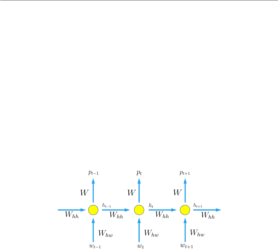
6 RECURRENT NEURAL NETWORK FOR SHORT TEXT CLASSIFICATION 35
6 Recurrent Neural Network for Short Text Classifica-
tion
We know that fully connected neural networks and CNNs can only process individual
inputs. The previous input and the following input are completely unrelated. However, in
some tasks we need to be able to better process the sequences, where the previous input
and the subsequent input are related. For example, if we want to understand a sentence,
it’s not enough to understand each word separately. We need to understand a group of
words or the entire sequence of words. So we need another very important neural network
in deep learning: recurrent neural network (RNN).
6.1 Vanilla Recurrent Neural Network
Figure 6.1: Recurrent neural network and the unfolding in time of the computation invol-
ved in its forward computation
Figure 6.1 shows a vanilla RNN being unfolded into a full network. By unfolding we mean
that we write out the network for the complete sequence. The parameters in RNN are as
follows: g and f are activation functions. w
t
is the input at time step t. h
t
is the hidden
layer state at time step t. We can think of the hidden state h
t
as the memory of the
network. p
t
is the output prediction at time step t. W
hw
is the weight matrix from input
layer to hidden layer. Here the first subscript h indicates that we want to work out the
hidden layer. The second subscript implies that matrx W
hw
multiplied by w
t
. Accordingly
W maps hidden layer to output layer. W
hh
is the weight matrix between hidden layers.
Note that a RNN shares the same set of parameters (W
hw
, W
hh
and W ) across all time
steps, thus greatly reducing the total number of parameters we need to learn.[3] At time
t:
h
t
= g(W
hh
h
t−1
+ W
hw
w
t
+ c) (6.1)
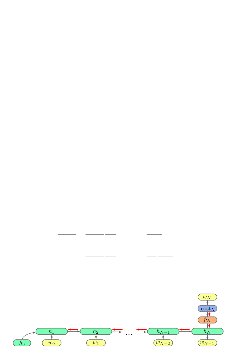
6 RECURRENT NEURAL NETWORK FOR SHORT TEXT CLASSIFICATION 36
p
t
= f(W h
t
+ b) (6.2)
The above formulas define the forward propagation in RNN. We define (W
hh
h
t−1
+W
hw
w
t
)
as V [h
t−1
, w
t
] to simplify the notations. We take the matrix W
hh
and W
hw
, put them side
by side and stack them horizontally as follows: [W
hh
.
.
. W
hw
] = V . Besides, [h
t−1
, w
t
]
indicates that we stack these two vectors vertically like
"
h
t−1
w
t
#
. To make it clearly, we say
h is 100 dimensional and w is 10,000 dimensional. Then W
hh
will be (100, 100) and W
hw
will be (100, 10000). When we stack these two matrices together, V will be a (100, 10100)
matrix. Correspondingly
"
h
t−1
w
t
#
will be a (10100, 100) vector. So [W
hh
.
.
. W
hw
] multiplied
by
"
h
t−1
w
t
#
we will get (W
hh
h
t−1
+ W
hw
w
t
). We rewrite the formula 6.1 and 6.2 as follows
for simplicity:
h
t
= g(V [h
t−1
, w
t
] + c) (6.3)
p
t
= f(W h
t
+ b) (6.4)
Exploding and vanishing gradients problems. We are interested in how the gradient
propagates back in time in RNN:
∂cost
N
∂h
1
=
∂cost
N
∂p
N
∂p
N
∂h
N
Y
n∈{N,...,2}
∂h
n
∂h
n−1
!
=
∂cost
N
∂p
N
∂p
N
∂h
N
Y
n∈{N,...,2}
∂h
n
∂z
n
∂z
n
∂h
n−1
!
(6.5)
Figure 6.2: Problem of exploding and vanishing gradients in RNN (adopted from [2])
6 RECURRENT NEURAL NETWORK FOR SHORT TEXT CLASSIFICATION 37
We define (W
hh
h
t−1
+ W
hw
w
t
+ c) in Formula 6.1 as z
n
. Then we get following derivatives:
∂h
n
∂z
n
= diag(g
0
(z
n
)) (6.6)
∂z
n
∂h
n−1
= W
hh
(6.7)
We rewrite the partial derivatives in Formula 6.5:
∂h
n
∂h
n−1
=
∂h
n
∂z
n
∂z
n
∂h
n−1
= diag(g
0
(z
n
)) W
hh
(6.8)
∂cost
N
∂h
1
=
∂cost
N
∂p
N
∂p
N
∂h
N
Y
n∈{N,...,2}
∂h
n
∂h
n−1
!
=
∂cost
N
∂p
N
∂p
N
∂h
N
Y
n∈{N,...,2}
diag(g
0
(z
n
)) W
hh
!
(6.9)
The core of the recurrent product is the repeated multiplication of W
hh
. If the largest
eigenvalue of W
hh
equals 1, then gradient will propagate and it will be stable; if it is
greater than 1, the product will grow exponentially as we multiply more and more times,
the gradients will explode; if it is less than 1, the product will shrink exponentially, the
gradients will vanish. These are problems in RNN: we will not be able to train the model
if it explodes because the gradients will be infinite; if it vanishes, we will not be able to
learn long range dependencies because we will get zero gradients after a few steps back
in time.
Solutions to exploding and vanishing gradients problems. In general, gradient ex-
plosion is easier to handle. Our program will receive a NaN error when gradient explodes.
We can also set a threshold, we can clip gradient values which exceed the preferred range
when gradient exceeds this threshold.
Gradient vanishing problem is more difficult to handle. We can use other types of RNNs,
such as LSTMs and gated recurrent unit (GRU), which is a most popular way and will
be discussed in the flowing paragraph.
We can also use new activation functions rectified linear unit (ReLU) instead of Sig-
moid and Tanh. See Table3.
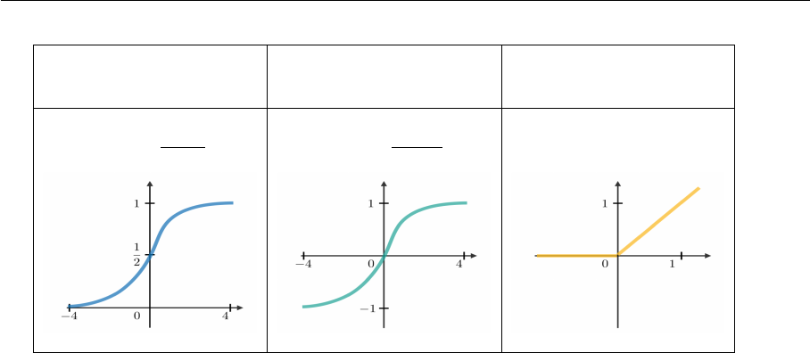
6 RECURRENT NEURAL NETWORK FOR SHORT TEXT CLASSIFICATION 38
Sigmoid Tanh ReLU
g(z) =
1
1+e
−z
g(z) =
e
z
−e
−z
e
z
+e
−z
g(z) = max(0, z)
Table 3: Commonly used activation functions
6.2 Long Short-Term Memory
When the time interval is large, it’s very difficult for simple RNNs to model long-distance
dependencies, known as long-term dependencies problem.[22][10] Long short-term memo-
ry (LSTM)[23] which was proposed by Hochreiter and Schmidhuber in 1997 has cleverly
solved this problem. LSTM networks – usually just called LSTMs, are a special kind of
RNN, capable of learning long-term dependencies.[4]
In the following paragraph we’ll step by step build a basic LSTMs model. Here we have
two time steps and we’re interested in how the hidden layer in the previous time step gets
updated into the next time step. The update equation is as follows:
h
n
= g(V [w
n−1
; h
n−1
] + c) (6.10)
Here h indicates hidden layers, w stands for input words and p is the output prediction.
As Figure 6.3 presents, when we go from h
n−1
to h
n
we are going to pass the hidden
layer h
n−1
and the input w
n−1
together through a linear transformation and a tanh non
linearity. This is a simple RNN architecture.
h
n
= tanh(V [w
n−1
; h
n−1
] + c) (6.11)
In the hidden layer of the original RNN there is only one hidden state, which is very
sensitive to short-term inputs. The next step is that we introduce an extra layer called
cell state c and we can think of it as our memory, we use it to store our long-term state.
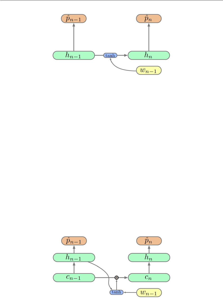
6 RECURRENT NEURAL NETWORK FOR SHORT TEXT CLASSIFICATION 39
Figure 6.3: Basic RNN architecture (adopted from [2])
We then promote the hidden layer h to upper layer as Figure 6.4 shows. We update the
cell state c
n
by taking the previous cell state c
n−1
and adding in a contribution from our
hidden layer h
n−1
with our input w
n−1
which looks just like previous simple RNN. The
difference is in this network we basically update cell states. And what really matters is
these updates are additive. In the simple recurrent network as we go from one hidden
layer to the next we are actually multiplying whereas in this network we do lots of sums.
When we differentiate the sum rather than the product, the gradient can flow nicely back
through the sum. The key thing in LSTMs is we replace multiplication with sum.
c
n
= c
n−1
+ tanh(V [w
n−1
; h
n−1
] + b
c
) (6.12)
h
n
= tanh(V [w
n−1
; h
n−1
] + c) (6.13)
Figure 6.4: The cell state of LSTM (adopted from [2])
The next thing we need to do is called gating. The idea of gating in neural networks is
just computing a non linearity which is bounded between 0 and 1 and we can think of it
like a switch: if it is 1 we turn on the connection, if it is 0 we turn it off. The key thing
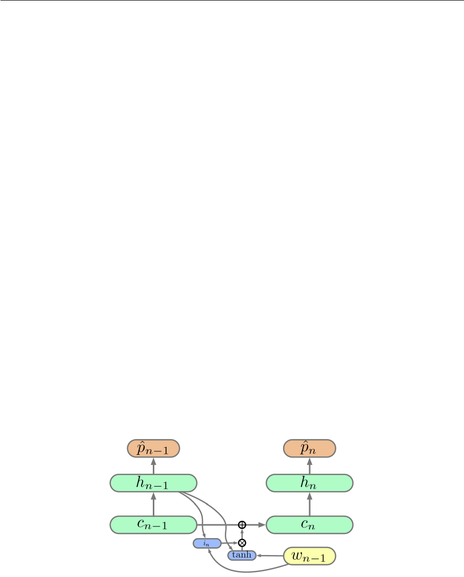
6 RECURRENT NEURAL NETWORK FOR SHORT TEXT CLASSIFICATION 40
is that it is a continous function so we can differentiate it and do back propagation. The
gate is actually a fully connected layer whose input is a vector and output is a vector
between 0 and 1. Suppose W is the weight matrix of the gate and b is the bias term. The
gate can be expressed as follows:
g(x) = σ(W x + b) (6.14)
As Figure 6.5 presents, here we introduce the input gate i. We gate the contribution
from the input and previous hidden layer. We then take a new linear transformation of
the input w
n−1
and the previous hidden layer h
n−1
, apply a sigmoid function to it and
get a vector of gates. When observing formula 6.15, we can think of it in this way. If the
gate is 1 then we will get a big contribution from our current input. If the gate is 0 then
we will get no contribution from current input, cell state c
n
is equal to cell state c
n−1
, so
there is no update and model forgets nothing. If a gate is closed for many time steps, we
will obtain long time dependencies. So input gate gives us the ability to ignore inputs.
c
n
= c
n−1
+ i
n
◦ tanh(V [w
n−1
; h
n−1
] + b
c
) (6.15)
i
n
= σ(W
i
[w
n−1
; h
t−1
] + b
i
) (6.16)
Figure 6.5: The input gate of LSTM (adopted from [2])
We have the ability either to include or ignore of the input but we do not have the ability
to forget things what are in our cell state. Now we add a forget gate f as in Figure 6.6.
As formula 6.19 shows, it is a sigmoid function of a new linear transformation of the input
w
n−1
and hidden layer h
n−1
. This forget gate is then multiplied by the previous cell state
c
n−1
to get a new cell state 6.17. Our new memory or new cell state is a mixture of the
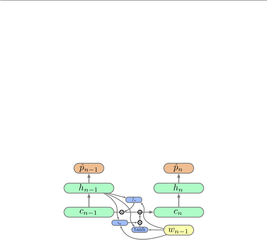
6 RECURRENT NEURAL NETWORK FOR SHORT TEXT CLASSIFICATION 41
previous cell state c
n−1
weighted by the forget gate f
n
and our new update from our input
and the previous hidden layer weighted by the input gate i
n
. If all the forget gates are set
to 0, we will forget all the memories. If all the input gates are set to 0, we will ignore all
the inputs. So the model can choose between do I really propagate information forward
perfectly and ignore inputs or do we forget what we have seen and introduce something
new.
c
n
= f
n
◦ c
n−1
+ i
n
◦ tanh(V [w
n−1
; h
n−1
] + b
c
) (6.17)
i
n
= σ(W
i
[w
n−1
; h
t−1
] + b
i
) (6.18)
f
n
= σ(W
f
[w
n−1
; h
t−1
] + b
f
) (6.19)
Figure 6.6: The forget gate of LSTM (adopted from [2])
Finally in LSTMs we always add a output gate o on the output from the cell state c
n
to the hidden layer h
n
, as in Figure 6.7.
h
n
= o
n
◦ tanh(W
h
c
n
+ b
h
) (6.20)
c
n
= f
n
◦ c
n−1
+ i
n
◦ tanh(V [w
n−1
; h
n−1
] + b
c
) (6.21)
i
n
= σ(W
i
[w
n−1
; h
t−1
] + b
i
) (6.22)
f
n
= σ(W
f
[w
n−1
; h
t−1
] + b
f
) (6.23)
o
n
= σ(W
o
[w
n−1
; h
t−1
] + b
o
) (6.24)
In summary, the hidden state h in RNN stores some historical information, which can be
regarded as a kind of memory. In a simple RNN, the hidden state is rewritten at each time
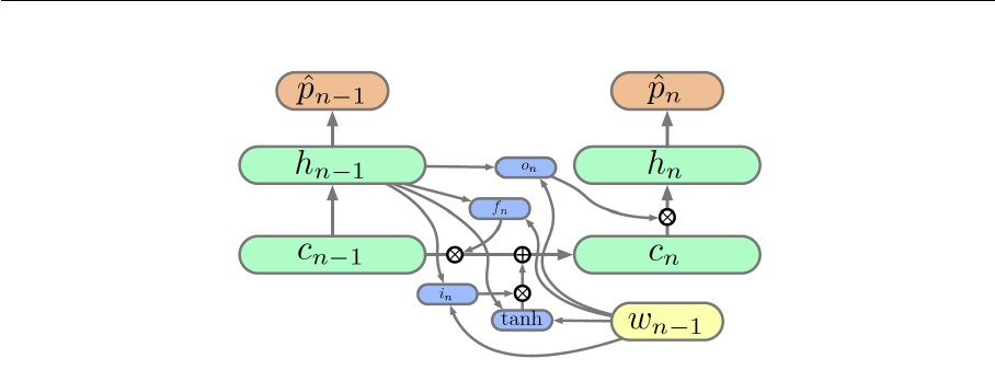
6 RECURRENT NEURAL NETWORK FOR SHORT TEXT CLASSIFICATION 42
Figure 6.7: The output gate of LSTM (adopted from [2])
step, so it can be seen as a short-term memory. In contrast, long-term memory in neural
networks can be seen as a network parameter, which is stored in the weight matrices. It
contains the information learned from training data, and its update cycle is much longer
than short-term memory.
In LSTMs, cell state c can capture some critical information and has the ability to keep
it for a certain time. The life cycle of the stored information in cell state c is longer
than short-term memory, but much shorter than long-term memory, so it is called long
short-term memory (LSTM).
6.3 Recurrent Convolutional Neural Network
In our work, we also experiment with recurrent convolutional neural network for text
classification (RCNN) proposed by Lai (2015). To present a word meaning better and
more precisely, we combine a word with its context. As shown in Figure 6.8, we use a
bidirectional recurrent neural network to capture contexts. As shown in equation 6.25
and 6.26, c
l
(w
i
) denotes the left context of word w
i
and c
r
(w
i
) denotes the right context
of word w
i
. e is a word embedding. W
(l)
, W
(r)
are matrices used to transfer contexts into
the next layer. W
(sl)
, W
(sr)
are matrices used to combine the context of the current word
with its left/right contexts.
c
l
(w
i
) = f(W
(l)
c
l
(w
i−1
) + W
(sl)
e(w
i−1
)) (6.25)
c
r
(w
i
) = f(W
(r)
c
r
(w
i+1
) + W
(sr)
e(w
i+1
)) (6.26)
Thus, the representation of word w
i
can be defined as a concatenation of word embedding
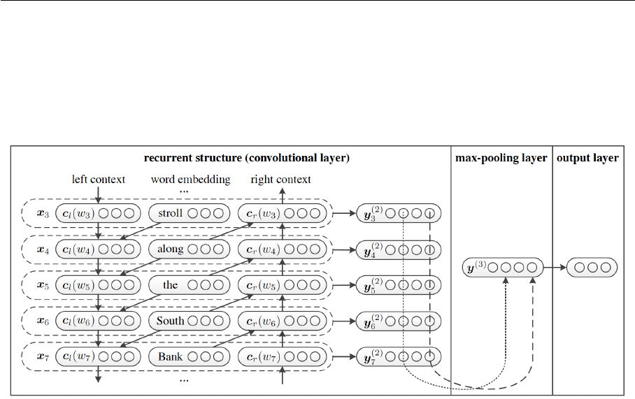
6 RECURRENT NEURAL NETWORK FOR SHORT TEXT CLASSIFICATION 43
e(w
i
), its left context vector c
l
(w
i
) and its right context vector c
r
(w
i
).
x
i
= [c
l
(w
i
); e(w
i
); c
r
(w
i
)] (6.27)
Figure 6.8: Recurrent convolutional neural network for text classification (adopted from
[33])
After we calculate the representation of each word w
i
, we can obtain the whole text
representation using equation 6.28.
y
(2)
i
= tanh(W
(2)
x
i
+ b
(2)
) (6.28)
So how do we extract features from texts? We simply apply a max-pooling layer after all
the word representations are calculated. Note that the max function is an element-wise
function. That is, the k-th element of y
(3)
is the maximum in the k-th elements of y
(2)
i
.
Therefore, we can convert sentences of different lengths into a fixed length vector. Mean-
while, we are also able to capture the most important textual information of documents.
y
(3)
=
n
max
i=1
y
(2)
i
(6.29)
7 EXPERIMENTS 45
7 Experiments
7.1 Data
We conduct our experiments on four widely used datasets: TREC, Twitter, AG News and
Movie Review. A summary of the datasets are listed in Table 4.
Datasets c l m train/test |V | |V
pre
|
TREC 6 10 33 5452/500 8602 7223
Twitter 3 19 35 9684/3547 20755 12140
AG News 4 7 23 120000/7600 38916 25310
Movie Review 2 21 59 10662/CV 19897 16394
Table 4: Summary statistics of datasets. c: number of target classes, l: average sentence
length, m: maximum sentence length, train/test: training/test set size, |V |: vocabulary
size, |V
pre
|: number of words present in the set of pre-trained word embeddings, CV: there
is no standard train/test split, thus 10-fold cross validation is used.
TREC. TREC
1
is a question answering dataset. This dataset is adopted from [Li et al.
2002][36]. It includes six different kinds of questions. TREC class descriptions are shown
in Table5. TREC details are listed in Table 6.
Abbreviation abbreviation or expression abbreviated
Entity food, animal, technique, language, plant, word, sport, etc.
Description definition or description of something, etc.
Human title or description of a person, etc.
Location city, state, country, etc.
Numeric count, date, size, weight, speed, temperature, distance, etc.
Table 5: Class descriptions of TREC dataset
Twitter. Twitter
2
is a dataset for a sentiment analysis competition. We need to predict
three labels: positive, negative and neutral. Because tweets are noisy, they are specially
preprocessed in our experiments, details can be seen in preprocessing part in this chapter.
Twitter details are listed in Table 7.
1
http://cogcomp.cs.illinois.edu/Data/QA/QC/
2
https://www.cs.york.ac.uk/semeval-2013/task2/

7 EXPERIMENTS 46
Abbreviation What is the full form of .com?
Entity What’s the second most used vowel in English?
Description What is an annotated bibliography?
Human Who is the founder of Scientology?
Location What is the highest waterfall in the United States?
Numeric How many people in the world speak French?
Table 6: Example sentences of TREC dataset
Positive
Good morning Becky! Thursday is going to be Fantastic!
T
aylor Swift is coming with Ed Sheeran June 29th, most perfect news I’ve
heard all night.
Neutral
The heat game may cost a lot, plus I would rather see Austin Rivers play.
N
ovember is an odd release date if true, but if it becomes big enough
maybe she could sing it at Grammys.
Negative
W
hy is it so hard to find the @TVGuideMagazine these days? Went to 3
stores for the Castle cover issue. NONE. Will search again tomorrow...
Just found a piece of candy that may have been injected with something.
Table 7: Example sentences of Twitter dataset
AG News. AG News is a collection of news articles. This dataset is adopted from [Zhang
et al., 2015][62]. The original data consists of class index (1 to 4), news title and news
description. We only use news title in our short text classification experiments. AG News
details can be seen in Table 8.
Sci/Tech IBM to hire even more new workers.
Sports Capacity crowds at beach volleyball rock the joint.
World US fighter squadron to be deployed in South Korea next month.
Business Staples profit up, to enter china market.
Table 8: Example sentences of AG News dataset
Movie Review. Movie Review
3
is a dataset used in sentiment analysis experiments. This
dataset is adopted from [Pang and Lee, 2005][42]. It contains sentences labeled with re-
spect to their overall sentiment polarity (positive or negative). Movie Review does not
have a standard test set. So for this dataset we randomly select 10% of the training data
3
http://www.cs.cornell.edu/people/pabo/movie-review-data/
7 EXPERIMENTS 47
as the dev set. Movie Review details can be seen in Table 9.
Positive
If this movie were a book, it would be a page-turner, you can’t wait to see
what happens next.
T
he film is faithful to what one presumes are the book’s twin premises - -
that we become who we are on the backs of our parents, but we have no
idea who they were at our age; and that time is a fleeting and precious
commodity no matter how old you are.
Negative
Too slow for a younger crowd, too shallow for an older one.
T
he problem is not that it’s all derivative, because plenty of funny movies
recycle old tropes. The problem is that van wilder does little that is
actually funny with the material.
Table 9: Example sentences of Movie Review dataset
7.2 Preprocessing
Text preprocessing is always the first step of a good NLP system, which provides the sys-
tem with clean, easy to handle forms. The impact on the performance of commonly used
text preprocessing methods with traditional machine learning classifiers has been investi-
gated in a previous work[53], which shows that appropriate combinations of preprocessing
methods depending on the domains and languages might result in a significant improve-
ment of the accuracy, whereas inappropriate combinations might decrease the accuracy as
well. A similar study with deep learning classifiers has also been conducted recently[11].
Therefore text preprocessing methods should be used and especially carefully selected.
In order to understand why text preprocessing really matters, we now consider the pre-
viously used sentences:
(1) I do not like this type of movie, but I like this one.
(2) I like this kind of movie, but I do not like this one.
We can clearly see that these two snippets represent completely opposite meanings. The
question is in what ways text preprocessing might affect our sense of how different they
are. To begin with, we calculate the cosine similarity of these two sentences, which is 0.90.
The relevant document frequency matrix are shown in Table 10 when considered only
lowercase words.
7 EXPERIMENTS 48
i do not like this type of movie but one kind
(1) 2 1 1 2 2 1 1 1 1 1 0
(2) 2 1 1 2 2 0 1 1 1 1 1
Table 10: Document term matrix with stop words retained
We then remove stop-words according to the natural language tool kit’s (NLTK) list of
English stop-words. With those removed, as shown in Table 11, the two snippets now look
less similar than before. In fact, the cosine distance between them decreases from 0.90
to 0.64. Thus, when asked how similar the two snippets are, our conclusions differ. And
this does matter because text similarity calculation is the core and foundation of unsu-
pervised learning techniques, such as clustering. Our observation of the above experiment
makes it clear that using different text preprocessing methods will lead to different results.
like type movie one kind
(1) 2 1 1 1 0
(2) 2 0 1 1 1
Table 11: Document term matrix with stop words removed
Next, the widely used text preprocessing techniques including lowercasing, tokenization,
stop-words removal, stemming and lemmatizing are introduced.
Lowercasing
There are two case conversion approaches, lowercasing and uppercasing. Here we only
focus on lowercasing, where all letters in all words of the document is converted comple-
tely to lowercase. The reason for doing this is that whether or not the first letter of a
word is uppercase typically does not affect its meaning.[17] For example, “Computer” and
“computer” all refer to the same type of machine which is able to be instructed to carry
out sequences of arithmetic or logical operations automatically. So it is unnecessary to
regard them as two different words in text analysis. Furthermore, it will lead to decline
in the accuracy without lowercasing under such circumstances. However, there is not a
general rule which demonstrates that lowercasing can always improve the performance.
Especially when our corpus is in German, it would be more appropriate to retain the
capitalization form of words since it is an important characteristic of German language.
In English only proper nouns such as the names of people, cities, countries, nationalities,
and languages, etc. are capitalized. From the following example we can notice that all

7 EXPERIMENTS 49
nouns are capitalized in German, wherever they appear in a sentence. This is a nearly
unique feature in a contemporary language.
EN: A computer is a machine that can be instructed to carry out sequences
of arithmetic or logical operations automatically.
DE: Ein Computer ist eine Maschine, die angewiesen werden kann, Sequenzen
von arithmetischen oder logischen Operationen automatisch auszuführen.
Tokenization
Tokenization methods consist of sentence tokenization and word tokenization. Sentence
tokenization is the process of splitting or segmenting text into individual sentences. Nor-
mally sentence tokenization is followed by word tokenization. Word tokenization is the
process of splitting or segmenting sentence into a list of words. The resulting word tokens
can be then used in further processing. Tokenization is important in NLP, especially in
the operations where each word needs to be individually dealed with such as stemming
and lemmatizing. In our work, we use NLTK library to tokenize words. Here is a word
tokenization example.
Original text:
He jumped in and swam to the opposite bank.
Tokenized text:
[‘He’, ‘jumped’, ‘in’, ‘and’, ‘swam’, ‘to’, ‘the’, ‘opposite’, ‘bank’]
Removing stop-words
Sometimes some extremely commonly used words are unlikely to convey us much useful
information, such as “the”, “the”, “and”, etc. These words are called stop-words. They can
be removed from texts and excluded from the vocabulary we built. Removing stop-words
has its benefit: we wouldn’t want the stop-words to take up too much space in our databa-
se or memory when processing large scale corpus. However it also has downsides, it might
affect the accuracy. There is no standard stop-words list. NLTK has a list of stop-words in
16 different languages. We can also define our own stop-words list according to our needs
in different domains and languages. In our experiments, stop-words are not removed.
Stemming and lemmatizing
Stemming and lemmatizing aims to reduce inflectional forms and sometimes derivational-
ly related forms of a word to a common base form.[38] Stemming refers to the process of
reducing a word to its most basic form. For instance, with removal of derivational affixes of
the following words, the verb “to jump” may appear as: “jumped”, “jumping” and “jumps”,

7 EXPERIMENTS 50
we can obtain their common base form: jump.
Lemmatizing or lemmatization refers to the process of conducting morphological ana-
lysis to correctly return the base form for each word, which here we call it lemma. For
instance, the verb ‘to swim’ may appear as: “swam”, “swum”, “swimming” and “swims”,
with lemmatizing we will obtain “swim” or “swimming” depending on the context, where
“swimming” can be either the base form of a noun “swimming-pool” or of a verb “I swam in
the river”. Whereas with stemming we might obtain “swim”. In fact, stemmer is typically
easier to implement and runs faster than lemmatizer, because stemmer simply operates on
a single word without any knowledge of the context but lemmatizer requires a dictionary
look-up operation.
By observing the raw tweets we can find that it is a quite noisy corpus. The language used
in tweets is very informal, with creative punctuation and spelling, misspellings, slang, new
words and genre-specific terminology and abbreviations. Tweets also have lots of special
characters such as emoticons, URLs, user-mentions, etc. as shown below. So we need some
additional special preprocessing methods for tweets. In our work, we adopt the methods
from a Kaggle twitter sentiment analysis competition
4
.
#NowPlaying Michael Jackson - She’s Out of My Life (Live At Wembley July
16. http://t.co/vxRYuADn L.O.V.E it! #MjTunes
URL
A uniform resource locator (URL), or web address in spoken English, is a reference to a
web resource which specifies its location. In our daily lives we would love to share content
such as URLs with friends or the public via Twitter. However URL in tweets doesn’t pro-
vide us with any valuable information in text classification tasks. One feasible approach is
removing all the URLs. Here we replace all the URLs in tweets with word URL. Note that
all the links (URLs) posted in tweets will automatically be processed and shortened. The
related regular expression used to match URLs is ((www\.[\S]+)|(https?://[\S]+)).
User mention
Lots of tweets have an associated symbol @. For example, we would like to mention our
friends with @username to share some funny posts or interesting ideas with them, or we
just want to let someone else know that we are talking about them. User mention does
not provide us with any useful information either. We replace all the user mentions in
tweets with word USER_MENTION. The regular expression used to match user mention is
4
https://github.com/abdulfatir/twitter-sentiment-analysis

7 EXPERIMENTS 51
@[\S]+.
Hashtag
A hashtag which is written with a # symbol, is used to index keywords or topics in tweets,
allowing us to easily follow or mention topics we are interested in. We simply replace all
the hashtags with the words with hash symbol #. For instance, #KIT is replaced with KIT.
The regular expression used to match hashtags is #(\S+).
Retweet
A retweet is a re-posting of a tweet. Sometimes we type RT at the beginning of a tweet to
indicate that we are re-posting someone else’s tweet. We remove RT from the tweets. The
regular expression used to match retweets is \brt\b.
Emoticon
Emoticon is a set of characters used in social media to express emotion or active atmos-
phere, etc. They are textual portrayals of our moods or facial expressions. There is a list
of commonly used emoticons on Wikipedia
5
. Exhaustively list and match all of the diffe-
rent emoticons that could possibly be used in tweets is obviously hard and impossible. In
our work, we just match some widely used emoticons. We replace the matched emoticons
with either EMO_POS, EMO_NEG or EMO_NEU depending on whether or not it’s positive. The
regular expressions used to match emoticons are listed in Table 12 and Table 13.
Type Emoticons
(1) Smiley :), : ), :-), (:, ( :, (-:
(2) Laughing :D, : D, :-D, xD, x-D, XD, X-D, 8D, 8-D, =D, =3
(3) Sad :-(, : (, :(, ):, ) :, )-:
(4) Surprise :-O, :O, :-o, :o
(5) Kiss <3, :*
(6) Wink ;-), ;), ;-D, ;D, (;, (-;
(7) Crying :,(, :’(, :"(
Table 12: List of some widely used emoticons
Besides, we convert 2 or more letter repetitions to two letters. For instance, someone use
tweets like “I loooooove it soooo much!” to emphasize the most significant words and
express their strong feelings. Here we convert this sentence to “I love it so much!”.
5
https://en.wikipedia.org/wiki/List_of_emoticons
7 EXPERIMENTS 52
Type Regex Replacement
(1) Smiley (:\s?\)|:-\)|\(\s?:|\(-:) EMO_POS
(2) Laughing (:\s?D|:-D|x-?D|X-?D|8-?D|=D|=3) EMO_POS
(3) Sad (:\s?\(|:-\(|\)\s?:|\)-:) EMO_NEG
(4) Surprise (:-?O|:-?o) EMO_NEU
(5) Kiss (<3|:\*) EMO_POS
(6) Wink (;-?\)|;-?D|\(-?;) EMO_POS
(7) Crying (:,\(|:\’\(|:"\() EMO_NEG
Table 13: List of regular expressions used to match emoticons
To have a better understanding of the preprocessing part, we select two original and pre-
processed sampled sentences listed below:
Before: @jackseymour11 I may have an Android phone by the time I get back
to school! :)
After: USERMENTION i may have an android phone by the time i get back
to school EMOPOS
Before: #NowPlaying Michael Jackson - She’s Out of My Life (Live At Wembley
July 16. http://t.co/vxRYuADn L.O.V.E it! #MjTunes
After: nowplaying michael jackson she is out of my life live at wembley
july 16 URL love it mjtunes
7.3 Evaluation Metrics
Binary classification
For a specific task, suppose we have a variety of machine learning or deep learning models
on hand. The question is: which model should we choose from all these available models
and apply it in the task? Actually all the machine learning algorithms consist of combi-
nations of just three components: representation, evaluation and optimization.[19] So it’s
important to choose proper evaluation metrics that match our tasks. We compute our
selected evaluation metric for multiple different models. Then we select the model with
best value of evaluation metric.
An evaluation function, or objective function, or scoring function, is used to distinguish
good classifiers from bad ones. Error rate and accuracy, they are two most commonly used
evaluation metrics in binary and multiclass classification tasks. Error rate is the ratio of

7 EXPERIMENTS 53
the number of samples with wrong predictions to the total number of samples. Accuracy
is the ratio of the number of samples with correct predictions to the total number of
samples.
Accuracy =
#correct predictions
#total instances
(7.1)
Error rate =
#wrong predictions
#total instances
(7.2)
However, these two metrics sometimes can not provide us with any accurate information
when the dataset has imbalanced classes, especially when greatly unbalanced. For instan-
ce, a dataset has 1000 randomly selected items in total, of which 990 are of class A and
only 10 are of class B. We build a classifier to predict relevant items, and see that its
accuracy on a test set is 99.0% which is amazingly good. But for comparison, suppose
we have a dummy classifier that does not look at the features at all, and always just
blindly predict the most frequent class (here class A). This dummy classifier’s accuracy
would also be 99.0%. It completely ignores the input data thus can not be used in practice.
For binary classification tasks, according to the combination of samples’ real categories
and our predicted categories, samples can be grouped into four classes: true positive (TP),
false positive (FP), true negative (TN) and false negative (FN). The confusion matrix is
shown in Table 14, where each row of the matrix represents the instances in an actual
class, while each column represents the instances in a predicted class.
True Positive TP FN
True Negative FP TN
Predicted Positive Predicted Negative
Table 14: Confusion matrix of binary classification
Precision and recall are then defined as:
precision =
T P
T P + F P
(7.3)
recall =
T P
T P + F N
(7.4)
Generally speaking, it is common that when the value of precision is higher, recall is often
lower. When the value of precision is lower, recall is often higher. For example, suppose
we are in a supermarket buying strawberries. We can get good strawberries as many as

7 EXPERIMENTS 54
possible by increasing the number of picked strawberries. If all the strawberries are se-
lected, then all the good strawberries must be selected, so precision would be lower. If
we want the proportion of good ones in the selected strawberries as high as possible, we
can only pick strawberries with most confidence, but this will inevitably leads to miss-
ing a lot of good strawberries, which makes recall lower. So there is always a trade-off
between precision and recall. In the recommendation system, in order to disturb users as
little as possible, it is more desirable that the recommended content is of users’ interest,
so precision is more important. In the fugitive information retrieval system, it is more
desirable to miss the fugitives as little as possible, so recall is crucial. Text classification
is a precision-oriented machine learning task, where we concern about how many positive
predicted documents are really positive.
A measure which combines precision with recall is the traditional F -measure or balanced
F -score. It is the harmonic mean of precision and recall.
F 1 =
2 × precision × recall
precision + recall
(7.5)
It is a special case of the general F (β) measure. F (β)-measure is the weighted harmonic
mean of precision and recall.
F (β) =
(1 + β
2
) × precision × recall
β
2
× precision + recall
(7.6)
Where β > 0 measures the relative importance of recall to precision. When β = 1, it
degenerates into the standard F 1 score, when β > 1, recall has a greater impact, when
β < 1, precision has a greater influence.
Multiclass classification
The situation is different in multiclass classification tasks. Each combination of two cate-
gories has a corresponding confusion matrix. The evaluation metric of multiclass classifi-
cation on N categories can be divided into N evaluation metrics of binary classification
on 2 categories.
The final evaluation metrics are averages across classes. There are two possible ways
that the metrics are averaged across all the classes. A straightforward approach is to
first calculate the precision and recall score on each confusion matrix. We record them as
(P
1
, R
1
), (P
2
, R
2
), . . . , (P
n
, R
n
), we then get the F 1
macro
score by working out the average.

7 EXPERIMENTS 55
P
macro
=
1
n
n
X
i=1
P
i
(7.7)
R
macro
=
1
n
n
X
i=1
R
i
(7.8)
F 1
macro
=
2 × P
macro
× R
macro
P
macro
+ R
macro
(7.9)
We can also work out the averages of T P , F P , T N, F N on each confusion matrix, record
them as T P , F P , T N, F N. Based on these averages, we can then calculate P
micro
, R
micro
and F1
micro
.
P
micro
=
T P
T P + F P
(7.10)
R
micro
=
T P
T P + F N
(7.11)
F 1
micro
=
2 × P
micro
× R
micro
P
micro
+ R
micro
(7.12)
As a comparison, each class has equal weight in macro scores whereas in micro scores each
instance has equal weight and largest classes have most influence. We compute metrics
within each class, average resulting metrics across classes to get macro scores. We ag-
gregrate outcomes across all classes, compute metrics with aggregate outcomes to obtain
micro scores. So how should we make a choice between macro and micro scores? If the
classes have about the same number of instances, macro and micro scores will be about
the same. If some classes are much larger or have more instances than others, and we want
to weight metric towards the largest ones, we use micro scores, if towards the smallest
ones, use macro scores. In our work, we compute confusion matrices and obtain the above
evaluation values with machine learning library for python called scikit-learn.
7.4 Computational Complexity
Here we consider the computational complexity of convolutional neural network for text
classfication.
Time complexity
The time complexity, also called computational complexity, describes the amount of ti-
me it takes to run an algorithm. Time complexity is normally calculated by counting the

7 EXPERIMENTS 56
number of elementary operations performed by the algorithms. In scientific computations,
the computational complexity of deep learning architectures such as TensorFlow or Py-
Torch is calculated by estimating the number of floating point operations (FLOPs) in the
forward pass. Here elementary operation refers to FLOPs, which includes multiplication
and accumulation. We ignore negligible costs such as non-linearities, dropout, and nor-
malization layers. How do we estimate FLOPs? The dot product of vectors and matrices
(matrix multiplication) is one of the most important operations in deep learning. Thus
matrix multiplication and matrix transpose are basic operations. Matrix multiplication
involves the accumulation of products or put it in another way, multiplier–accumulator
(MAC) operations. The number of OPs/s (the number of operations per second) can be
estimated by counting how many MACs can be completed per second. Each multiplication
and accumulation is considered to be 1 OP, so 1 MAC is actually 2 OPs.
To compute the number of FLOPs, we assume convolution is implemented as a sliding
window. For a standard convolutional kernel in a single layer we have:
Time ∼ O
2 · K
2
· M
2
· C
in
· C
out
(7.13)
where M is the height and width of the output Feature Map, K is the Kernel width
(assumed to be symmetric), C
in
is the number of channels of the input feature maps or
the number of output channels in the previous convolutional layer. C
out
is the number of
output channels or the number of output feature maps in this convolution layer.
To illustrate the above equation, we can analysis it in this way. We modify formula 7.4:
Time ∼ O
2 · C
in
· K
2
· M
2
· C
out
!
(7.14)
We first calculate the number of operations of one pixel in an output feature map. Then it
is multiplied by (M
2
· C
out
) to be generalized to the entire output feature maps. The part
in the parentheses can be divided into two steps as shown in equation 7.15, where the first
item denotes we count the number of multiplications and the second denotes the number
of accumulations. Because bias is not considered, we add 1 and finally get (2 · C
in
· K
2
)
as shown in formula 7.14.
(2 · C
in
· K
2
− 1) = (C
in
· K
2
) + (C
in
· K
2
− 1) (7.15)

7 EXPERIMENTS 57
In addition, the size of output feature map M is determined by the size of input feature
map X, kernel width K, padding and stride, which can be estimated as follows:
M = (X − K + 2 ∗ Padding)/Stride + 1 (7.16)
The total time complexity of all convolutional layers is:
Time ∼ O
2 ·
D
X
l=1
M
2
l
· K
2
l
· C
l−1
· C
l
!
(7.17)
where l is the index of a convolutional layer, and D is the model depth or the number
of convolutional layers. M
l
is the spatial size of the output feature map. K
l
is the spatial
size (length) of the filter. C
l
is the number of filters (width) or the output channels in the
l-th layer. C
l−1
denotes the number of input channels of the l-th layer or the number of
output filters in the (l − 1)-th layer.
The theoretical time complexity in above equations are simply the estimations of neural
networks, rather than the actual running time. Because the actual running time are sen-
sitive to implementations and hardwares.[21]
Space complexity
Space complexity is a measurement of the amount of working storage an algorithm needs.
It means how much memory, in the worst case, is needed at any point in the algorithm. In
practical deep learning, often the size of neural networks is bound by available memory.
Sometimes there could possibly be a situation that can evolve where the memory can
not hold so many model weights and intermediate variables that the program crashes.
Therefore it is necessary to know how to calculate the size of the graphics card’s memory
occupied by the model that we design together with the intermediate variables. Then we
will be comfortable with the memory of graphics card and the problems and bugs that it
arises.
The space complexity in deep learning includes two parts: total parameters and output
feature maps in each layers. Total parameters are the total weight parameters of the all
layers where there are model parameters (the first part of the formula below). Feature
maps are the output feature maps calculated in each layer of the model (the second part
of the formula below).

7 EXPERIMENTS 58
Space ∼ O
D
X
l=1
K
2
l
· C
l−1
· C
l
+
D
X
l=1
M
2
· C
l
!
(7.18)
As we can see in formula 7.18, total parameters is only related to the spatial size of the
kernel K, the number of channels C and the number of convolutional layers D, regardless
of the input size (weight sharing). In fact, practical memory usage also depends on the
implementations and platforms.
7.5 Entity Linking
We use TagMe
6
to extract and obtain useful named entities. TagMe[20] is a powerful sys-
tem which has the ability to properly identify meaningful substrings (also called spots) in
a plain-text and link each of them to a closely related Wikipedia
7
page fast and efficiently.
Besides TagMe, there are also some other entity linking tools such as Dexter
8
, Babelfy
9
,
etc. We choose to use TagMe in our work because it is reported to be one of the best entity
linking tool in the scientific community. Most importantly, compared with existing tools,
TagMe is able to annotate short texts such as tweets, search-engine results, news titles, etc.
An annotation is a pair (spot, entity), where spot (also mention) is a substring of the
input text, and entity is a reference to the Wikipedia page that represents the meaning
of the spot in that context. In a proper case, not only can the mention (spot) be linked
to a named entity which contains the right mention in respect of named entity linking
(NEL), but also solves the important and pervasive semantic problems across languages,
ambiguity and polysemy, in the sense of word sense disambiguation (WSD).
We use RESTful API to obtain annotations provided by TagMe. We first send a text to
the server for example. The response of the server includes all the annotations found in
that text. TagMe associates an attribute with each annotation, called ρ. This ρ value,
which estimates the goodness of the annotation with respect to other entities existing in
the input text, should be used as a filter to discard annotations that are below a given
threshold. A reasonable threshold is reported to be between 0.1 and 0.3. Note that ρ does
not indicate the relevance of the entity in the input text, but is rather a confidence score
assigned by TagMe to that annotation.
6
https://tagme.d4science.org/tagme/
7
https://en.wikipedia.org/wiki/Main_Page
8
http://dexter.isti.cnr.it/
9
http://babelfy.org/

7 EXPERIMENTS 59
For instance, consider the following sentence:
On this day 24 years ago Maradona scored his infamous Hand of God goal
against England in the quarter-final of the 1986.
For this short text, the extracted annotations in JSON format are given below:
1 {
2 "test": "5",
3 "annotations": [
4 {
5 "spot": "On this day",
6 "link_probability": 0.0014018691144883633,
7 "rho": 0.0576556958258152,
8 "title": "BBC News Online"
9 },
10 {
11 "spot": "day",
12 "link_probability": 0.0030609103851020336,
13 "rho": 0.02183143049478531,
14 "title": "Martin Day"
15 },
16 {
17 "spot": "24 years",
18 "link_probability": 0.0019907099194824696,
19 "rho": 0.0009953549597412348,
20 "title": "1986 FIBA World Championship"
21 },
22 {
23 "spot": "Maradona",
24 "link_probability": 0.15395480394363403,
25 "rho": 0.2147175818681717,
26 "title": "Diego Maradona"
27 },
28 {
29 "spot": "infamous",
30 "link_probability": 0.022769613191485405,
31 "rho": 0.011384806595742702,
32 "title": "Infamous (Motionless in White album)"
33 },
34 {
35 "spot": "Hand of God goal",
36 "link_probability": 0.8918918967247009,
37 "rho": 0.582613468170166,
38 "title": "Argentina v England (1986 FIFA World Cup)"

7 EXPERIMENTS 60
39 },
40 {
41 "spot": "England",
42 "link_probability": 0.2987603545188904,
43 "rho": 0.27085503935813904,
44 "title": "England national football team"
45 },
46 {
47 "spot": "quarter-final",
48 "link_probability": 0.014687774702906609,
49 "rho": 0.1550503820180893,
50 "title": "2010 FIFA World Cup knockout stage"
51 }
52 ]
53 }
The ρ value of the recognized spot “On this day” which links to Wikipedia page “BBC
News Online” is 0.06. The ρ value of spot “Maradona” which links to entity “Diego Ma-
radona” is 0.21. The latter annotation looks more reasonable in this sentence and thus
should have and actually does have a higher ρ value. In fact, “Maradona”, the well-known
football player “Diego Maradona”, is a partial name which have to be linked to the ap-
propriate entity in a KB, such as Wikipedia or DBpedia.
In our work, we set ρ to 0.1. As a result, in this example, “Diego Maradona”, “Argen-
tina v England (1986 FIFA World Cup)”, “England national football team” and “2010
FIFA World Cup knockout stage” are considered to be proper named entities and will be
used in the next experimental steps.
In our experiments, we find that not all the sentences have extracted named entities.
Not all the named entities have correlated entity embeddings in Wikipedia2Vec. To de-
monstrate that named entities can be a useful feature, some statistics are listed in Table 15.
We fisrt use TagMe to get named entities. From Table 15 we can know that about 92%
sentences in TREC have entities. We then query these entities in Wikipedia2Vec to obtain
entity embeddings. About 98% extracted named entities have corresponding entity em-
beddings in Wikipedia2Vec. Moreover, 92% sentences have at least one entity embedding,
which means that only 8% sentences do not have features. These statistics make it clear
that extracted named entities can be regarded as a new feature which will be utilized in
our work. Feature statitics on the other datasets can be viewed in Appendix. For those
entities which do not have entity embeddings, they are zero initialized.
7 EXPERIMENTS 61
TREC Training Set Test Set
#total sentences 5452 500
#sentences with entity 5031 460
#sentences without entity 421 40
percentage of sentences with entity 92% 92%
#total entities 12291 874
#average entities per sentence 2.44 1.90
#total entities with entity embedding in Wikipedia2Vec 12020 856
percentage of entities with entity embedding 98% 98%
#sentences which have at least 1 entity embedding 5000 460
percentage of sentences which have at least 1 entity embedding 92% 92%
Table 15: Feature statistics on TREC
7.6 Experimental Setup
Word Embeddings
The Word2Vec
10
model takes a document corpus as input and produces the word vectors
as output. It is pre-trained on a very large unannotated corpus so we are able to achieve
better generalization when given limited amount of training data. The pre-trained vectors
of word2vec model are trained on part of Google News dataset which contains about 100
billion words. The model contains 300 dimensional vectors for 3 million words and phra-
ses. Words which do not present in the set of pre-trained vectors are randomly initialized
from a uniform distribution [−0.25, 0.25].
The Wikipedia2Vec models are trained on an English Wikipedia dump. Available pre-
trained models which have 100, 300 and 500 dimension words and entities can be found
on the Wikipedia2Vec official page
11
. We can also train our own model using the latest
English Wikipedia dump
12
.
We can train the Doc2Vec model of the English Wikipedia dump. Detailed training in-
troductions can be followed on this page
13
. In our work, the model size is set to 300 and
epochs 5. We can improve the model accuracy with with more training epochs, such as
10 or 20 epochs, but it would take much more training time.
10
https://code.google.com/archive/p/word2vec/
11
https://wikipedia2vec.github.io/wikipedia2vec/pretrained/
12
https://dumps.wikimedia.org/enwiki/
13
https://markroxor.github.io/gensim/static/notebooks/doc2vec-wikipedia.html

7 EXPERIMENTS 62
Hyperparameters
Parameters Values
filter sizes lower:[3, 4, 5], upper:[3, 4, 5, 6]
number of filters lower:16, upper:256
dropout rate 0.5
batch size 64
l2 regularization 3.0
embedding dimension lower:100, upper:300
learning rate 0.005
Table 16: Experiment hyperparameters
Experimental Environment
In our work, all the experiments are accomplished on a workstation containing 3.60GHz
Intel Xeon 4 Cores CPUs, 1 single NVIDIA GeForce GTX 1060 GPU with use of CUDA
10.0.130, cuDNN 7.3.0 and TensorFlow 1.3.
7.7 Results and Analysis
Our experimental results are listed in Table 17. All the experiments are repeated three to
five times under the optimal hyperparameters. We then take an average of the results as
final result. As we can see, our TextCNN implementation gets almost the same or better
performance as our baseline. Our model EntCNN has higher accuracy with maximum
1.4% improvement than our baseline model TextCNN on all datasets. This conveys the
information that entities do help to improve the performance of text classification.
The accuracy on Twitter 68.1% is much lower than three other datasets. It can be at-
tributed to the following reasons. First, Twitter, which contains less than ten thousand
sentences, is not a large corpus, especially for deep learning. Second, Twitter is a set of
tweets which has three labels. Besides, it contains longer, more complicated and noisy
sentences. When compared with TREC and AG News, it is obviously more difficult to
analyze and label the sentences. Third, Twitter is a dataset used for sentiment analysis
task but we do not conduct any similar analysis in our work. As reported in the original
sentiment analysis competition paper [41], the best result of SemEval-2013 Task 2 subtask
B is 69%, so our result appears to be reasonable.

7 EXPERIMENTS 63
Model Twitter TREC Movie Review AG News
Baseline(Word2Vec) 57.24 89.33 81.52 86.11
Word(Word2Vec) 68.1 89.4 83.0 87.4
Word(Word2Vec) + Entity(Wikipedia2Vec) 68.2 90.4 83.0 87.9
Word(Wikipedia2Vec) + Entity(Wikipedia2Vec) 68.8 89.8 82.8 87.9
∆ + 0.7 + 1.0 - + 0.5
Word(Doc2Vec) 69.3 91.6 81.5 87.6
Word(Word2Vec) + Entity(Doc2Vec) 68.0 89.0 82.0 88.1
Word(Doc2Vec) + Entity(Doc2Vec) 69.3 93.0 81.3 87.4
∆ - + 1.4 +0.5 +0.5
Entity(Wikipedia2vec) 46.4 61.4 51.8 79.3
Word(BERT) 69.3 90.2 79.3 87.4
Table 17: Classification results of different models on several different datasets. Baseline:
we take the results reported in [55] as our baseline. Word: TextCNN(i.e. text classification
using only words). Word + Entity: EntCNN(i.e. text classification using words and
entities). Entity: text classification using only entities. All the words and entities are
initialized from 300 dimensional pre-trained models Word2Vec, Wikipedia2Vec, Doc2Vec
and 768 dimensional BERT respectively.
To verify the hypothesis that we can benefit from entities, we conduct an experiment whe-
re we use only entities to classify documents. The experimental results in Table 17 confirm
that by using only entities, we are already able to achieve an accuracy that is better than
randomly guessing (50% for binary classification and 33% for three-class classification).
From the confusion matrices shown in Figure 7.1 and Figure 7.2, we can find that our
model EntCNN improves the classification accuracy on label HUM from 91% to 95%, ENTY
from 73% to 77% respectively, and has overall higher accuracy than TextCNN. That is,
named entities do help us to classify sentences on label HUM and ENTY. Another observation
about the classification results is that labels ABBR and ENTY have much lower accuracy
than other labels. One possible explanation is that label ABBR and ENTY are lack of enough
training data. Confusion matrices on the other datasets can be seen in Appendix.
We also compare the classification performance when we use different pre-trained word
vector models. The entity vectors are initialized with Wikipedia2Vec or Doc2Vec. We
do not use pre-trained Word2Vec model to initialize entity vectors because it is trained
with Google News articles rather than Wikipedia dump, so pre-trained vectors do not be
available for many Wikipedia entities. The word vectors of different models are initialized
with Word2Vec, Wikipedia2Vec and Doc2Vec models respectively. From the results shown
in Table 17, it is clear that the choice of pre-trained word vector models has an impact
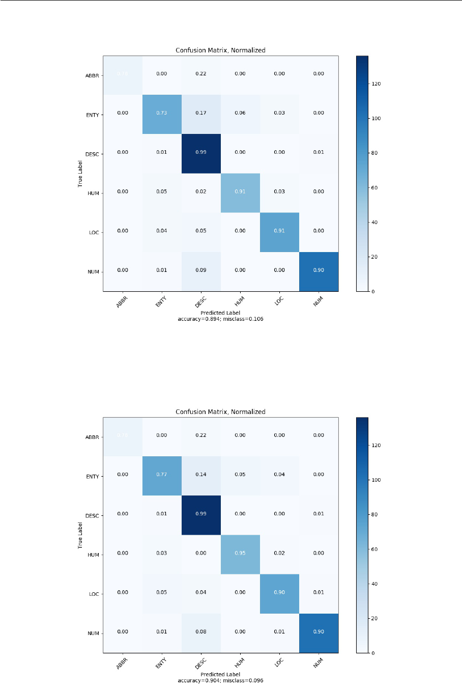
7 EXPERIMENTS 64
Figure 7.1: Baseline model (TextCNN) normalized confusion matrix on TREC
Figure 7.2: Our model (EntCNN) normalized confusion matrix on TREC

7 EXPERIMENTS 65
on performance, however different models perform better for different datasets. Doc2Vec
works better for Twitter and TREC. Word2Vec and Wikipedia2Vec work better for Movie
Review. All of them have good performance on AG News. So there is no single optimal
choice for all datasets. Practically, our results suggest experimenting with different pre-
trained word vectors for new datasets.
We also conduct an experiment where we initialize words from state-of-the-art model
BERT. The word vetors in BERT have 768 dimensions. We obtain word vectors from an
open toolkit bert-as-service
14
. The results demonstrate that we can not further improve
the classification performance by just using word vectors from BERT.
To demonstrate that our preprocessing methods on Twitter do help us to improve the
classification accuracy, we conduct an experiment with and without tweets specific pre-
processing methods. By comparing the results shown in Table 18, we can clearly find that
our preprocessing methods improve the classification accuracy by average 2% ∼ 3%. 2%
is not a small number generally, especially when considering the fact that our model has
an improvement of average 1%. This suggests that preprocessing is always the first step
to consider and extremely important in NLP. When we conduct our experiments, we find
that there is a performance difference when applying different preprocessing techniques
on the same task.
Dataset Without With
Word(Word2Vec) 66.1 68.1
Word(Word2Vec) + Entity(Wikipedia2Vec) 66.1 68.2
Word(Wikipedia2Vec) + Entity(Wikipedia2Vec) 65.5 68.8
Table 18: Comparison between different preprocessing methods on Twitter. Without:
classification without tweets specific preprocessing. With: classification with tweets spe-
cific preprocessing.
We also compare the performance of different text classification models, see Table 19.
As we can see, TextCNN is already able to achieve pretty good performance, the models
proposed later do not have much improvement. From evaluation scores on AG News and
TREC listed in Tables at the end of this chapter, we can see on what labels the classifi-
cation accuracy is improved.
14
https://github.com/hanxiao/bert-as-service
7 EXPERIMENTS 66
To summarize our experimental results, our model EntCNN can improve the classificati-
on performance on four datasets, no matter they are traditional multi-class classification
tasks or sentiment analysis tasks where we want to determine whether a sentence is po-
sitive or negative. Experimental results demonstrate that entities provide us with more
contextual information and thus can help to classify documents.
Model Twitter TREC Movie Review AG News
TextCNN 68.1 89.4 83.0 87.4
RCNN 67.6 90.4 82.3 88.3
Bi-LSTM 63.6 88.4 83.7 88.2
Table 19: Comparison between different models. TextCNN: Convolutional Neural Net-
work for sentence classification (Kim, 2014). RCNN: Recurrent Covolutional Neural Net-
work for text classification (Lai, 2015). All words are initialized from 100 dimensional
pre-trained model GloVe respectively.
Dataset Precision Recall F1-Score
World 90.5 87.4 88.9
Sports 90.3 94.5 92.3
Business 84.9 85.2 85.0
Sci/Tech 86.5 85.1 85.8
Table 20: Evaluation of EntCNN on AG
News
Dataset Precision Recall F1-Score
World 91.5 85.7 88.5
Sports 89.0 95.2 92.0
Business 82.4 86.4 84.4
Sci/Tech 88.8 82.9 85.3
Table 21: Evaluation of TextCNN on AG
News
Dataset Precision Recall F1-Score
ABBR 100 77.8 87.5
ENTY 90.0 76.6 82.8
DESC 83.4 98.6 90.4
HUM 92.5 95.4 94.0
LOC 92.4 90.1 91.3
NUM 98.1 90.3 94.0
Table 22: Evaluation of EntCNN on TREC
Dataset Precision Recall F1-Score
ABBR 100 77.8 87.5
ENTY 89.6 73.4 80.7
DESC 80.5 98.6 88.6
HUM 90.8 90.8 90.8
LOC 93.7 91.4 92.5
NUM 99.0 90.3 94.4
Table 23: Evaluation of TextCNN on TREC

8 CONCLUSION 67
8 Conclusion
8.1 Summary
Text classification has always been considered to be extremely important in NLP rese-
arch and industry community. However, short text classification has not been a popular
research topic. Thus, in our work, we explore the possibility to utilize named entities in
neural network architectures to classify documents. Our key contribution is that we are
the first to demonstrate that named entities help us to improve the performance of short
text classification.
In our work, a novel neural network based approach of short text classification is proposed.
We utilize and modify the convolutional neural network for text classification (TextCNN)
proposed by Kim (2014)[28]. Our model is not only trained on top of pre-trained word
vectors, but also on top of pre-trained entity vectors. Tagme is utilized to extract named
entities from documents. We utilize Wikipedia2Vec and Doc2Vec to get entity vectors.
Our feature statistics on four popular used NLP datasets demonstrate that the extracted
named entities can be a feature for the following work. We compare the performance of
our proposed model EntCNN with the baseline model TextCNN. By comparing our ex-
perimental results of different models on different datasets, we can conclude that entity
vectors are helpful on mutil-class classification tasks. The impact of different kinds of
pre-trained word vector representations on the classification accuracy is also studied in
this work. The relative performance achieved using Word2Vec, Wikipedia2Vec, Doc2Vec
and BERT depends on the dataset. Our results suggests that we experiment with dif-
ferent pre-trained word vectors for new NLP tasks. Additionally, our applied intensive
preprocessing methods on tweets have been proven to show great improvement on the
classification performance. Therefore, our experiment suggests that corpus specific pre-
processing is always considered to be a crucial step in NLP.
8.2 Future Work
Our work is based on TextCNN proposed by Kim in 2014. This model achieves good
classification performance across a wide range of text classification tasks and has beco-
me a standard baseline for text classification architectures since then. However fantastic
progress has been achieved in NLP since last year in 2018. Large scale pre-trained lan-
guage representation models like BERT, GPT and ELMo using the enormous amount of
unannotated text on the web are proposed. These models can then be fine-tuned on small

8 CONCLUSION 68
amount of data NLP tasks and have been proven to be state-of-the-art models. BERT
is a milestone in NLP and will have a lasting impact on subsequent NLP research and
industrial applications. So in the following work, our efforts should be focused on these
new SOTA models. Generative pre-trained language models together with task-specific
fine-tuning should be considered to be a general NLP framework.
Due to time and compute resource reasons we did not explore fine-tuning BERT for text
classification. Especially, according to our literature review, BERT for short text classi-
fication has not been studied yet. How to learn better pre-trained representations will
continue to be a research popular point for some time. Pre-training on what size (word,
sub-word, character etc.), what kind of language model (LSTMs, Transformer, etc.) to
train, and how to adapt pre-trained models to specific tasks are interesting topics that
still need to be explored.
When BERT involved in our work, we could explore the possibility to combine BERT
input embeddings with entity embeddings. That is, BERT input representations are the
sum of the token embeddings, the segmentation embeddings, the position embeddings and
the entity embeddings.

A FEATURE STATISTICS 69
A Feature Statistics
Table 24: Feature statistics on Movie Review
Movie Review Positive Negative
#total sentences 5331 5331
#sentences with entity 4517 4379
#sentences without entity 814 952
percentage of sentences with entity 85% 82%
#total entities 14171 13014
#average entities per sentence 3.14 2.97
#total entities with entity embedding in Wikipedia2Vec 13827 12677
percentage of entities with entity embedding 98% 97%
#sentences which have at least 1 entity embedding 4455 4328
percentage of sentences which have at least 1 entity embedding 84% 81%
Table 25: Feature statistics on AG News
AG News Training Set Test Set
#total sentences 120000 7600
#sentences with entity 110719 6989
#sentences without entity 9281 611
percentage of sentences with entity 92% 92%
#total entities 323517 20626
#average entities per sentence 2.92 2.95
#total entities with entity embedding in Wikipedia2Vec 316591 20204
percentage of entities with entity embedding 98% 98%
#sentences which have at least 1 entity embedding 110001 6942
percentage of sentences which have at least 1 entity embedding 92% 91%
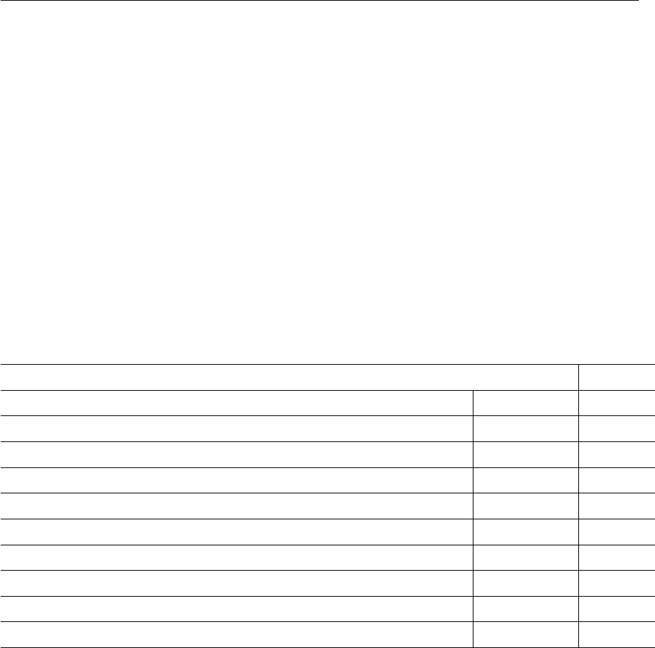
A FEATURE STATISTICS 70
Twitter Training Set Test Set
#total sentences 9684 3547
#sentences with entity 9219 3382
#sentences without entity 465 165
percentage of sentences with entity 95% 95%
#total entities 30551 10916
#average entities per sentence 3.31 3.23
#total entities with entity embedding in Wikipedia2Vec 28983 10278
percentage of entities with entity embedding 95% 94%
#sentences which have at least 1 entity embedding 9148 3345
percentage of sentences which have at least 1 entity embedding 94% 94%
Table 26: Feature statistics on Twitter
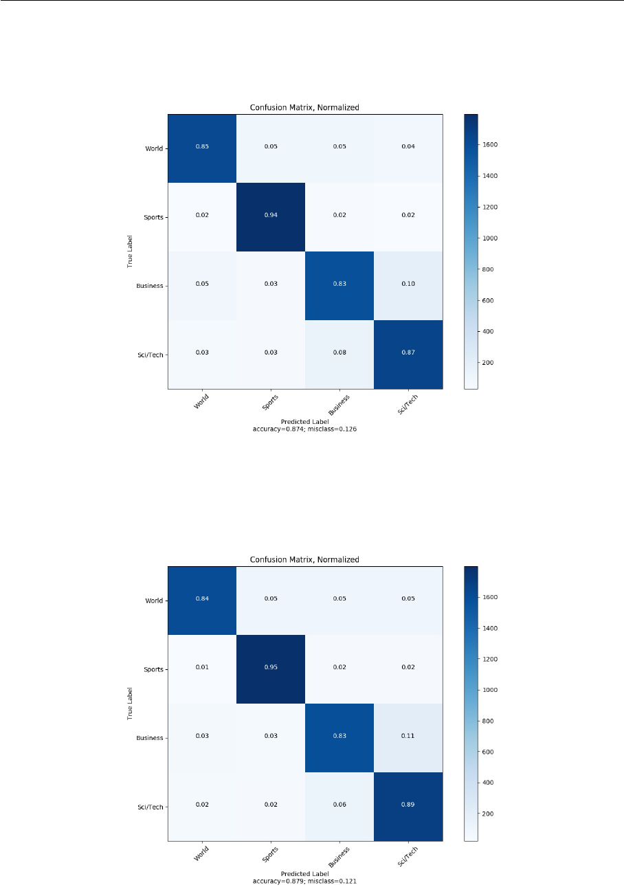
B CONFUSION MATRICES 71
B Confusion Matrices
Figure B.1: Baseline model (TextCNN) normalized confusion matrix on AG News
Figure B.2: Our model (EntCNN) normalized confusion matrix on AG News
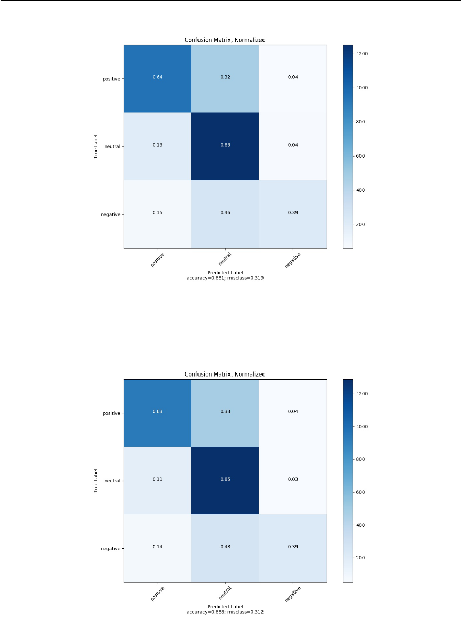
B CONFUSION MATRICES 72
Figure B.3: Baseline model (TextCNN) normalized confusion matrix on Twitter
Figure B.4: Our model (EntCNN) normalized confusion matrix on Twitter

LITERATUR 73
Literatur
[1] Attention in long short-term memory recurrent neural
networks. https://machinelearningmastery.com/
attention-long-short-term-memory-recurrent-neural-networks/. Acces-
sed: 2017-06-30.
[2] Deep learning for natural language processing. https://github.com/
oxford-cs-deepnlp-2017/lectures.
[3] Recurrent neural networks tutorial, part 1 – intro-
duction to rnns. http://www.wildml.com/2015/09/
recurrent-neural-networks-tutorial-part-1-introduction-to-rnns/.
Accessed: 2015-09-17.
[4] Understanding lstm networks. https://colah.github.io/posts/
2015-08-Understanding-LSTMs/.
[5] Visualizing what convnets learn. http://cs231n.github.io/understanding-cnn/.
[6] Aggarwal, C. C., and Zhai, C. A survey of text classification algorithms. In
Mining Text Data, C. C. Aggarwal and C. Zhai, Eds. Springer, 2012, pp. 163–222.
[7] Bahdanau, D., Cho, K., and Bengio, Y. Neural machine translation by jointly
learning to align and translate, 2014. cite arxiv:1409.0473Comment: Accepted at
ICLR 2015 as oral presentation.
[8] Bellman, R., and Collection, K. M. R. Adaptive Control Processes: A Guided
Tour. Princeton Legacy Library. Princeton University Press, 1961.
[9] Bengio, Y., Ducharme, R., Vincent, P., and Janvin, C. A neural probabilistic
language model. J. Mach. Learn. Res. 3 (Mar. 2003), 1137–1155.
[10] Bengio, Y., Simard, P., and Frasconi, P. Learning long-term dependencies
with gradient descent is difficult. Trans. Neur. Netw. 5, 2 (Mar. 1994), 157–166.
[11] Camacho-Collados, J., and Pilehvar, M. T. On the role of text preproces-
sing in neural network architectures: An evaluation study on text categorization and
sentiment analysis. CoRR abs/1707.01780 (2017).
[12] Chang, A., Spitkovsky, V. I., Manning, C. D., and Agirre, E. A comparison
of named-entity disambiguation and word sense disambiguation. In Proceedings of
the Tenth International Conference on Language Resources and Evaluation (LREC
2016) (Paris, France, may 2016), N. C. C. Chair), K. Choukri, T. Declerck, S. Goggi,

LITERATUR 74
M. Grobelnik, B. Maegaard, J. Mariani, H. Mazo, A. Moreno, J. Odijk, and S. Pipe-
ridis, Eds., European Language Resources Association (ELRA).
[13] Chorowski, J. K., Bahdanau, D., Serdyuk, D., Cho, K., and Bengio, Y.
Attention-based models for speech recognition. In Advances in Neural Information
Processing Systems 28, C. Cortes, N. D. Lawrence, D. D. Lee, M. Sugiyama, and
R. Garnett, Eds. Curran Associates, Inc., 2015, pp. 577–585.
[14] Conneau, A., Schwenk, H., Barrault, L., and LeCun, Y. Very deep convo-
lutional networks for natural language processing. CoRR abs/1606.01781 (2016).
[15] Dai, A. M., Olah, C., and Le, Q. V. Document embedding with paragraph
vectors. In NIPS Deep Learning Workshop (2015).
[16] Dash, M., and Liu, H. Feature selection for classification. Intell. Data Anal. 1, 3
(May 1997), 131–156.
[17] Denny, M. J., and Spirling, A. Text preprocessing for unsupervised learning:
Why it matters, when it misleads, and what to do about it. Political Analysis 26, 2
(2018), 168–189.
[18] Devlin, J., Chang, M., Lee, K., and Toutanova, K. BERT: pre-training of
deep bidirectional transformers for language understanding. CoRR abs/1810.04805
(2018).
[19] Domingos, P. A few useful things to know about machine learning. Commun. ACM
55, 10 (Oct. 2012), 78–87.
[20] Ferragina, P., and Scaiella, U. Tagme: On-the-fly annotation of short text
fragments (by wikipedia entities). In Proceedings of the 19th ACM International Con-
ference on Information and Knowledge Management (New York, NY, USA, 2010),
CIKM ’10, ACM, pp. 1625–1628.
[21] He, K., and Sun, J. Convolutional neural networks at constrained time cost. In
2015 IEEE Conference on Computer Vision and Pattern Recognition (CVPR) (June
2015), pp. 5353–5360.
[22] Hochreiter, S. Untersuchungen zu dynamischen neuronalen Netzen. Diploma the-
sis, Institut für Informatik, Lehrstuhl Prof. Brauer, Technische Universität München,
1991.
[23] Hochreiter, S., and Schmidhuber, J. Long short-term memory. Neural Comput.
9, 8 (Nov. 1997), 1735–1780.

LITERATUR 75
[24] James, G., Witten, D., Hastie, T., and Tibshirani, R. An Introduction to
Statistical Learning: With Applications in R. Springer Publishing Company, Incor-
porated, 2014.
[25] Joulin, A., Grave, E., Bojanowski, P., and Mikolov, T. Bag of tricks for
efficient text classification. CoRR abs/1607.01759 (2016).
[26] Jurafsky, D., and Martin, J. H. Speech and Language Processing (2Nd Edition).
Prentice-Hall, Inc., Upper Saddle River, NJ, USA, 2009.
[27] Kalchbrenner, N., Grefenstette, E., and Blunsom, P. A convolutional
neural network for modelling sentences. CoRR abs/1404.2188 (2014).
[28] Kim, Y. Convolutional neural networks for sentence classification. CoRR ab-
s/1408.5882 (2014).
[29] Kowsari, K., Meimandi, K. J., Heidarysafa, M., Mendu, S., Barnes, L. E.,
and Brown, D. E. Text classification algorithms: A survey. CoRR abs/1904.08067
(2019).
[30] Král, P. Named entities as new features for czech document classification. In
Proceedings of the 15th International Conference on Computational Linguistics and
Intelligent Text Processing - Volume 8404 (Berlin, Heidelberg, 2014), CICLing 2014,
Springer-Verlag, pp. 417–427.
[31] Krizhevsky, A., Sutskever, I., and Hinton, G. E. Imagenet classification with
deep convolutional neural networks. In Advances in Neural Information Processing
Systems 25, F. Pereira, C. J. C. Burges, L. Bottou, and K. Q. Weinberger, Eds.
Curran Associates, Inc., 2012, pp. 1097–1105.
[32] Kumar, A., Irsoy, O., Ondruska, P., Iyyer, M., Bradbury, J., Gulrajani,
I., Zhong, V., Paulus, R., and Socher, R. Ask me anything: Dynamic memory
networks for natural language processing. In Proceedings of The 33rd International
Conference on Machine Learning (New York, New York, USA, 20–22 Jun 2016),
M. F. Balcan and K. Q. Weinberger, Eds., vol. 48 of Proceedings of Machine Learning
Research, PMLR, pp. 1378–1387.
[33] Lai, S., Xu, L., Liu, K., and Zhao, J. Recurrent convolutional neural networks for
text classification. In Proceedings of the Twenty-Ninth AAAI Conference on Artificial
Intelligence (2015), AAAI’15, AAAI Press, pp. 2267–2273.
[34] Le, Q., and Mikolov, T. Distributed representations of sentences and documents.
In Proceedings of the 31st International Conference on International Conference on
Machine Learning - Volume 32 (2014), ICML’14, JMLR.org, pp. II–1188–II–1196.

LITERATUR 76
[35] Lee, C., and Lee, G. G. Information gain and divergence-based feature selection
for machine learning-based text categorization. Inf. Process. Manage. 42, 1 (Jan.
2006), 155–165.
[36] Li, X., and Roth, D. Learning question classifiers. In Proceedings of the 19th
International Conference on Computational Linguistics - Volume 1 (Stroudsburg,
PA, USA, 2002), COLING ’02, Association for Computational Linguistics, pp. 1–7.
[37] Liu, P., Qiu, X., and Huang, X. Recurrent neural network for text classification
with multi-task learning. CoRR abs/1605.05101 (2016).
[38] Manning, C. D., Raghavan, P., and Schütze, H. Introduction to Information
Retrieval. Cambridge University Press, New York, NY, USA, 2008.
[39] Mikolov, T., Chen, K., Corrado, G., and Dean, J. Efficient estimation of
word representations in vector space. CoRR abs/1301.3781 (2013).
[40] Mikolov, T., Sutskever, I., Chen, K., Corrado, G. S., and Dean, J. Distri-
buted representations of words and phrases and their compositionality. In Advances
in Neural Information Processing Systems 26, C. J. C. Burges, L. Bottou, M. Wel-
ling, Z. Ghahramani, and K. Q. Weinberger, Eds. Curran Associates, Inc., 2013,
pp. 3111–3119.
[41] Nakov, P., Rosenthal, S., Kozareva, Z., Stoyanov, V., Ritter, A., and
Wilson, T. SemEval-2013 task 2: Sentiment analysis in twitter. In Second Joint
Conference on Lexical and Computational Semantics (*SEM), Volume 2: Proceedings
of the Seventh International Workshop on Semantic Evaluation (SemEval 2013) (At-
lanta, Georgia, USA, June 2013), Association for Computational Linguistics, pp. 312–
320.
[42] Pang, B., and Lee, L. Seeing stars: Exploiting class relationships for sentiment ca-
tegorization with respect to rating scales. In Proceedings of the 43rd Annual Meeting
on Association for Computational Linguistics (Stroudsburg, PA, USA, 2005), ACL
’05, Association for Computational Linguistics, pp. 115–124.
[43] Peters, M., Ruder, S., and Smith, N. A. To tune or not to tune? adapting
pretrained representations to diverse tasks. CoRR abs/1903.05987 (2019).
[44] Peters, M. E., Neumann, M., Iyyer, M., Gardner, M., Clark, C., Lee,
K., and Zettlemoyer, L. Deep contextualized word representations. CoRR ab-
s/1802.05365 (2018).
[45] Radford, A. Improving language understanding by generative pre-training.

LITERATUR 77
[46] Řehůřek, R., and Sojka, P. Software Framework for Topic Modelling with Large
Corpora. In Proceedings of the LREC 2010 Workshop on New Challenges for NLP
Frameworks (Valletta, Malta, May 2010), ELRA, pp. 45–50. http://is.muni.cz/
publication/884893/en.
[47] Ristoski, P., and Paulheim, H. Rdf2vec: Rdf graph embeddings for data mining.
In The Semantic Web - ISWC 2016 : 15th International Semantic Web Conference,
Kobe, Japan, October 17-21, 2016, Proceedings, Part I (Cham, 2016), vol. 9981,
Springer International Publishing, pp. 498–514.
[48] Rush, A. M., Chopra, S., and Weston, J. A neural attention model for abstrac-
tive sentence summarization. In Proceedings of the 2015 Conference on Empirical
Methods in Natural Language Processing (Lisbon, Portugal, Sept. 2015), Association
for Computational Linguistics, pp. 379–389.
[49] Salton, G., Wong, A., and Yang, C. S. A vector space model for automatic
indexing. Commun. ACM 18, 11 (Nov. 1975), 613–620.
[50] Shen, W., Wang, J., and Han, J. Entity linking with a knowledge base: Issues,
techniques, and solutions. IEEE Transactions on Knowledge and Data Engineering
27, 2 (Feb 2015), 443–460.
[51] Srivastava, N., Hinton, G., Krizhevsky, A., Sutskever, I., and Salak-
hutdinov, R. Dropout: A simple way to prevent neural networks from overfitting.
Journal of Machine Learning Research 15 (2014), 1929–1958.
[52] Sutskever, I., Vinyals, O., and Le, Q. V. Sequence to sequence learning
with neural networks. In Advances in Neural Information Processing Systems 27,
Z. Ghahramani, M. Welling, C. Cortes, N. D. Lawrence, and K. Q. Weinberger, Eds.
Curran Associates, Inc., 2014, pp. 3104–3112.
[53] Uysal, A. K., and Gunal, S. The impact of preprocessing on text classification.
Inf. Process. Manage. 50, 1 (Jan. 2014), 104–112.
[54] Vaswani, A., Shazeer, N., Parmar, N., Uszkoreit, J., Jones, L., Gomez,
A. N., Kaiser, L., and Polosukhin, I. Attention is all you need. CoRR ab-
s/1706.03762 (2017).
[55] Wang, J., Wang, Z., Zhang, D., and Yan, J. Combining knowledge with deep
convolutional neural networks for short text classification. In Proceedings of the 26th
International Joint Conference on Artificial Intelligence (2017), IJCAI’17, AAAI
Press, pp. 2915–2921.

LITERATUR 78
[56] Xu, K., Ba, J., Kiros, R., Cho, K., Courville, A., Salakhudinov, R., Ze-
mel, R., and Bengio, Y. Show, attend and tell: Neural image caption generation
with visual attention. In Proceedings of the 32nd International Conference on Ma-
chine Learning (Lille, France, 07–09 Jul 2015), F. Bach and D. Blei, Eds., vol. 37 of
Proceedings of Machine Learning Research, PMLR, pp. 2048–2057.
[57] Yamada, I., Asai, A., Shindo, H., Takeda, H., and Takefuji, Y. Wiki-
pedia2vec: An optimized tool for learning embeddings of words and entities from
wikipedia. CoRR abs/1812.06280 (2018).
[58] Yamada, I., Shindo, H., Takeda, H., and Takefuji, Y. Joint learning of
the embedding of words and entities for named entity disambiguation. CoRR ab-
s/1601.01343 (2016).
[59] Yang, Z., Yang, D., Dyer, C., He, X., Smola, A., and Hovy, E. Hierarchical
attention networks for document classification. In Proceedings of the 2016 Conference
of the North American Chapter of the Association for Computational Linguistics:
Human Language Technologies (San Diego, California, June 2016), Association for
Computational Linguistics, pp. 1480–1489.
[60] Zeng, J., Li, J., Song, Y., Gao, C., Lyu, M. R., and King, I. Topic memory
networks for short text classification. In Proceedings of the 2018 Conference on Empi-
rical Methods in Natural Language Processing (Brussels, Belgium, 2018), Association
for Computational Linguistics, pp. 3120–3131.
[61] Zhang, X., and LeCun, Y. Which encoding is the best for text classification in
chinese, english, japanese and korean? CoRR abs/1708.02657 (2017).
[62] Zhang, X., Zhao, J. J., and LeCun, Y. Character-level convolutional networks
for text classification. CoRR abs/1509.01626 (2015).
[63] Zhang, Y., and Wallace, B. C. A sensitivity analysis of (and practitioners’ guide
to) convolutional neural networks for sentence classification. CoRR abs/1510.03820
(2015).
Erklärung
Ich versichere wahrheitsgemäß, die Arbeit selbstständig verfasst, alle benutzten Hilfsmittel
vollständig und genau angegeben und alles kenntlich gemacht zu haben, was aus Arbeiten
anderer unverändert oder mit Abänderungen entnommen wurde sowie die Satzung des KIT
zur Sicherung guter wissenschaftlicher Praxis in der jeweils gültigen Fassung beachtet zu
haben.
Karlsruhe, 29. August 2019 QINGYUAN BIE
