Variable Ratio Matching with Fine Balance in a Study of the Peer

Health Exchange



Samuel D. Pimentel



Frank Yoon



Luke Keele



June 25, 2015

Abstract

In some observational studies of treatment eﬀects, matched samples are created so

treated and control groups are similar in terms of observable covariates. Traditionally such

matched samples consist of matched pairs. However, alternative forms of matching may

have desirable features. One strategy that may improve eﬃciency is to match a variable

number of control units to each treated unit. Another strategy to improve balance is to

adopt a ﬁne balance constraint. Under a ﬁne balance constraint, a nominal covariate is

exactly balanced, but it does not require individually matched treated and control subjects

for this variable. Here, we propose a method to allow for ﬁne balance constraints when

each treated unit is matched to a variable number of control units, which is not currently

possible using existing matching network ﬂow algorithms. Our approach uses the entire

number to ﬁrst determine the optimal number of controls for each treated unit. For each

stratum of matched treated units, we can then apply a ﬁne balance constraint. We then

demonstrate that a matched sample for the evaluation of the Peer Health Exchange, an

intervention in schools designed to decrease risky health behaviors among youths, using a

variable number of controls and ﬁne balance constraint is superior to simply using a variable

ratio match.

Keywords: Matching; Fine Balance; Observational Study; Optimal Matching; Entire Number



For comments and suggestions, we thank Paul Rosenbaum. Research for this paper was conducted with

Government support under FA9550-11-C-0028 and awarded by the Department of Defense, Army Research Oﬃce,

National Defense Science and Engineering Graduate (NDSEG) Fellowship, 32 CFR 168a.



University of Pennsylvania, Philadelphia, PA, Email: spi@wharton.upenn.edu



Mathematica Policy Research, Princeton, NJ, Email: fyoon@mathematica-mpr.com



Penn State University, University Park, PA and the American Institutes for Research, Washington D.C.,

Email: [email protected].

This is the peer reviewed version of the following article: Pimentel, S.D., Yoon, F., and Keele, L.

(2015). "Variable-ratio matching with fine balance in a study of the Peer Health Exchange."

Statistics in Medicine, 34 (30) 4070-4082. doi:10.1002/sim.6593, which has been published in

final form at http://onlinelibrary.wiley.com/doi/10.1002/sim.6593/full. This article may be used for

non-commercial purposes in accordance with Wiley Terms and Conditions for Self-Archiving.

1 Introduction

1.1 A Motivating Example: Peer Health Exchange

Many under-resourced high schools lack any curriculum on health education. Health education

courses cover such topics as sexual health, substance abuse, and instruction on nutrition and

physical ﬁtness. Peer Health Exchange (PHE) is a nonproﬁt organization established in 2003

that seeks to provide health education in underprivileged high schools that lack such a curriculum

[1, 2]. Instead of providing curricular materials to schools, the PHE relies on a speciﬁc model

of health education. Schools that partner with PHE oﬀer health education through the use of

trained college student volunteers. College student volunteers serve as peer health educators for

high or middle school students. Using peer educators to address sensitive topics such as sexual

health is thought to allow for a stronger connection between the students and educators. The

PHE model is designed to modify student behaviors and attitudes in the areas of substance abuse

(use of alcohol, tobacco, and illicit drugs), sexual health (use of contraception, pregnancy, sexual

health risks), and mental health. The eﬀectiveness of the PHE model has not been rigorously

tested. Early research has shown that peer health educators can be more eﬀective than community

health nurses [3, 4]. A review of extant research by Kim and Free [5] found that peer-led sex

education improved knowledge, attitudes, and intentions, but actual sexual health outcomes were

not improved.

As part of a larger multiphase study to evaluate the eﬀectiveness of the PHE model, schools

in a large Midwestern city were recruited to implement the PHE model. At the same time a

set of comparison schools were selected via a pairwise Mahalanobis match and recruited into the

study. Schools were matched on covariates such as enrollment, the percentage of students eligible

to participate in the free or reduced price lunch program, the percentage of African American

students, and average test scores.

Within these schools, students completed a battery of survey items on health behaviors before the

PHE curriculum was implemented in the treated schools. The PHE curriculum was implemented in

the treated schools during the Spring semester of 2014. In total 121 students completed the PHE

curriculum. From the control schools, a pool of 357 students were available as controls. Hereafter,

we interchangeably refer to treated students as “PHE” students. Outcomes are to be measured

through a follow up survey to be administered in the summer of 2015. The follow-up survey is

to be based on the same battery of items on health behaviors measureded at baseline.

Even though the schools that did not receive the PHE curriculum were similar to those schools

that did, the study design also called for matching students at the individual level. The student-

level match was included since diﬀering outcomes among students may reﬂect initial diﬀerences

in student-level covariates between the treated and control groups rather than treatment eﬀects

[6, 7]. Pretreatment diﬀerences amongst subjects come in two forms: those that have been

accurately measured, which are overt biases, and those that are unmeasured but are suspected

to exist which are hidden biases. Matching methods are frequently used to remove overt biases.

Matched samples are constructed by ﬁnding close matches to balance pretreatment covariates

[8]. Ideally, such matches are constructed using an optimization algorithm [9–12]. One important

advantage of matching is that statistical adjustments for overt biases be done without references

to outcomes. This prevents explorations of the data that may invalidate inferential methods [13].

In fact, Rubin [14] recommends that analysts always remove outcomes until statistical adjustments

for observed confounders are complete. In the PHE study, outcomes were not available at the

time of this writing, but we can still consider how to best adjust for overt biases between treated

and control groups.

1.2 An Initial Pair Match

This article discusses a new matching method. To motivate this new method, however, we begin

by describing the balance on covariates before matching students and after an initial pair match.

In all, 21 covariates were available describing student demographics and behaviors in four health-

related subject areas. Table 1 shows means and absolute standardized diﬀerences in means, the

absolute value of the diﬀerence in means divided by the standard deviation before matching, for

the unmatched sample. Before matching, the PHE students were much more likely to be African

American, less likely to be female, and more likely to be eligible for the free or reduced price

lunch program. The measure of eligibility for the free lunch program is a key covariate as it is

the sole indicator of socio-economic status for the students in the study, and it is substantially

imbalanced with a standardized diﬀerence of 0.616 in the unmatched data. PHE students were

also more likely to have a higher incidence of drug use and sexual activity.

To reduce overt bias due to these imbalances, we ﬁrst implemented a pair match following which

might be considered standard practice in the literature following Rosenbaum [15, ch 8]. For

this match, we sought to minimize distances based on a robust Mahalanobis distance metric.

We also applied a caliper to the estimated propensity score through a penalty function. The

caliper restricts the absolute distance between a treated unit and potentially matched control.

For example, on the propensity score distance, a caliper penalizes or forbids a match between

two units whose estimated propensity scores diﬀer by more than the width of the caliper. We

set the caliper to be 0.5 times the standard deviation of the estimated propensity score. See

Rosenbaum [15, ch 8] for an overview of both the distance metric and calipers enforced via

penalties. We estimated the propensity score using a logistic regression model with a linear and

additive speciﬁcation. We implemented this match using the pairmatch function in Hansen’s

[2007] optmatch library in R.

For a number of measures, survey responses were missing. To understand, whether this pattern

of missingness diﬀered across the treated and control groups, we use a method recommended

by Rosenbaum [15]. Under this procedure, we imputed missing values using the mean for that

covariate, but we then created a separate indicator for whether the value was missing. We

then checked balance on these measures of missingness to understand whether the patterns

of missingness were imbalanced across treated and control groups. This approach is desirable

because it focuses on the limited goal of balancing observed patterns of missingness. As such it

does not require additional assumptions about the missingness mechanism that would be required

under most methods of multiple imputation.

Table 1: Summary of covariate balance for unmatched data and a pair match for PHE evaluation.

–St-diﬀ– = absolute standardized diﬀerence.

Unmatched Pair Match

Mean C Mean T –St-diﬀ– Mean C Mean T –St-diﬀ–

Demographics

African American 1/0 0.580 0.802 0.470 0.868 0.802 -0.140

Multi-Racial 1/0 0.008 0.033 0.206 0.008 0.033 0.207

White 1/0 0.160 0.008 -0.472 0.008 0.008 0.000

Hispanic 1/0 0.143 0.149 0.017 0.107 0.149 0.117

Female 1/0 0.669 0.463 -0.432 0.570 0.463 -0.224

Disability type 1 1/0 0.042 0.033 -0.046 0.025 0.033 0.042

Disability type 2 1/0 0.011 0.017 0.048 0.008 0.017 0.074

Disability type 3 1/0 0.252 0.198 -0.046 0.149 0.198 0.042

Free or reduced price lunch 1/0 0.641 0.917 0.630 0.950 0.917 -0.075

Substance Abuse History

Marijuana use 1/0 0.096 0.208 0.342 0.140 0.208 0.206

Drunk in past 30 days 1/0 0.096 0.151 0.178 0.067 0.151 0.272

5 or more drinks in past 30 days 0.014 0.034 0.147 0.000 0.034 0.250

Drug use past 30 days 0.140 0.322 0.477 0.223 0.322 0.260

Number of drug types used (0–10) 0.235 0.512 0.285 0.231 0.512 0.289

Sexual Behaviors

Number of sexual partners 0.172 0.458 0.326 0.347 0.458 0.127

Ever had sex 1/0 0.154 0.349 0.503 0.263 0.349 0.222

Understand cause of pregnancy 1/0 0.812 0.757 -0.139 0.709 0.757 0.121

Can obtain contraception 1/0 0.406 0.440 0.071 0.438 0.440 0.004

Perception of sex safety 3.034 2.944 -0.150 2.945 2.944 -0.002

Other Items

Decision-making skill 3.084 3.048 -0.075 3.083 3.048 -0.073

Knowledge of healthy eating 0.882 0.799 -0.319 0.817 0.799 -0.068

Number of times eating healthy 2.447 2.507 0.057 2.446 2.507 0.058

Number of days physically active 3.692 4.129 0.192 4.008 4.129 0.053

We report means and absolute standardized diﬀerences after the pair match in Table 1. Table 1

omits summaries for the missing data indicators. Those results are reported in the Supplementary

Materials along with plots of the propensity score distributions. Although the results from the

pair match are an improvement over the unmatched data, the balance statistics are still less

than satisfactory, as a number of signiﬁcant imbalances remained. Of the 21 covariates, 11 still

had imbalances in which the standardized diﬀerence exceeded 0.10, with the largest standardized

diﬀerence being 0.33. The ﬁve largest absolute standardized diﬀerences averaged 0.27. A general

rule of thumb is that matched standardized diﬀerences should be less than 0.20 and preferably

0.10 [15]. Is a better match possible?

1.3 Alternatives to the Initial Pair Match

We might seek to improve on the initial pair match in two ways. First, a substantial amount of

overt bias remains. That is, a number of covariates display imbalances that are larger than would

be produced in a randomized experiment. Second, we might seek to make greater use of the

controls. In the PHE data, there are nearly 3 times as many controls as treated units, and most

of those controls are discarded in a pair match. The use of additional controls can produce more

eﬃcient treatment eﬀect estimates. While eﬃciency may be a secondary concern in observational

studies, our goal is to produce an acceptable level of balance while using as much of the data as

possible to increase eﬃciency.

To further reduce overt bias in the match, a number of diﬀerent strategies are available. These

strategies include checking for a lack of common support, exact matching on covariates, using

penalty terms, or using ﬁne and near-ﬁne balance constraints. Fine balance forces exact balance

at all levels of a nominal variable but places no restriction on individual matched pairs—any one

treated subject can be matched to any one control [17]. For example, a ﬁne balance constraint

could require the same number of men and women be selected in the overall control group as

in the overall treated group, but in the resulting match men might be matched to women and

vice versa in individual pairs. Fine balance is not always possible and when this occurs near-ﬁne

balance is one alternative [18].

Fine balance constraints may be especially useful in the PHE evaluation match. Matching in

observational studies balances covariates stochastically, but may not have much success in bal-

ancing many small strata on discrete covariates because such imbalances can occur by chance.

When this is the case, ﬁne balance is often an eﬀective way to remove biases of important prog-

nostic covariates that may have a nonlinear eﬀect on the outcome. In the PHE evaluation match,

eligibility for the free lunch program is an important prognostic variable (as the sole proxy for

socio-economic status). Although it is reasonably well balanced by the pair match, its interac-

tions with other important variables may not be, and these are likely to be diﬃcult to balance

stochastically. Fine balance provides a natural way to balance such interactions.

While improving balance is one goal in a match, we might also wish to improve eﬃciency. To

improve eﬃciency, we can match with multiple controls. Under a matching with multiple controls,

each treated subject is matched to at least one control and possibly more. We can match with

multiple controls in three ways. First, given the treated control ratio in the PHE data, we could

match every treated unit to two controls. Alternatively, we could match with a variable ratio of

controls where the number of matched controls possibly varies for each treated unit. Matching

with a variable number of controls often removes more overt bias than matching with a ﬁxed ratio

of controls [10]. Another alternative would be a full match. A full match is the most general form

of optimal matching [11, 15, 19]. Under full matching, we create matched sets in which each

matched set has either 1 treated unit and a variable number of controls or 1 control unit with a

variable number of treated units. Full matching is the most general form of matching. Both a

pair match and any match with multiple controls are special cases of a full match [19].

Given the need to remove additional overt bias and the ratio of treated to control units in the

PHE data, one possible design for the PHE evaluation would be based on either a full match

or a variable control:treatment ratio match to make greater use of control units with ﬁne or

near-ﬁne balance to reduce overt bias. However, most matching algorithms do not allow one to

implement either a full match or a variable control:treatment ratio match with ﬁne or near-ﬁne

balance constraints.

For example, one widely used optimal matching algorithm is based on ﬁnding a minimum cost ﬂow

in a network. Hansen’s [2007] optmatch library in R uses an algorithm developed by Bertsekas

[20] that solves the minimum cost ﬂow problem. The fullmatch function in this library allows

for both full matches and variable ratio matches, but does not allow for ﬁne or near-ﬁne balance.

Other popular matching algorithms such as Coarsened Exact Matching [21] and Genetic Matching

[22] are also unable to perform a match of this type. It is possible to implement a variable ratio

match with ﬁne balance using integer programming [12]. However, software for integer based

matching is not widely available and scalability for matching in very large datasets is often more

diﬃcult. Below we develop a new algorithm that uses network ﬂows to minimize the total distance

among treated and control units in a variable-ratio match, but also allows for ﬁne or near-ﬁne

balance constraints.

1.4 Outline

The article is organized as follows. Section 2 develops notation and reviews variable-ratio matching

and ﬁne balance in greater detail. In particular, we introduce the entire number, a form of design-

based variable-ratio matching that will make incorporation of ﬁne balance constraints possible

[23]. In Section 3 we detail the proposed algorithm. We ﬁrst build intuition in Section 3.1

and then describe the general procedure in Section 3.2. Next, we demonstrate the use of our

method with the PHE evaluation data in Section 4. We then compare this match to two more

conventional matches. Section 5 concludes.

2 Review and Deﬁnitions of Variable-Ratio Matching, the

Entire Number, and Fine Balance

We begin with a review of variable-ratio matching via the “entire number.”

2.1 Review: Variable-Ratio Matching and the Entire Number

To ﬁx the concept of a variable-ratio match, we ﬁrst deﬁne some notation. A match consists of

i D 1; : : : ; I matched sets. Each matched set i may contain at least n

 2 subjects indexed

by j D 1; : : : ; n

. Within the matched set, we use an indicator Z

to denote exposure to the

PHE treatment, where Z

D 1 if a student attended the PHE program and Z

D 0 if the

student does not. Under the most general matching, there are m

students with Z

D 1 and

 m

D l

students where Z

D 0 (with m

and l

> 0). Under variable-ratio matching, we

ﬁx m

D 1 within each matched set, and l

is allowed to vary from matched set to matched set.

For each set i, we may also require each treated student to be matched to at least ˛  1 and

at most ˇ  ˛ controls, i.e. ˛  l

 ˇ. If ˛ D ˇ D 1, the matched set is a pair match.

If we set ˇ D 3 and ˛ D 1 each treated unit may be matched to 1,2 or 3 controls. Often we

place an upper limit on ˇ since there are rapidly diminishing returns on eﬃciency as ˇ increases

[11]. In general there is little to gain from ˇ D 10 and generally ˇ D 5 is suﬃcient. See Ming

and Rosenbaum [10] for a more detailed discussion of the gains from larger matched sets. Under

variable-ratio matching, the size of n

is permitted to vary with i, and we wish to select the size

of each l

to minimize a distance criterion. Ming and Rosenbaum [24] presented one algorithm

to select the size of each matched set. One alternative to their algorithm for selection of l

uses

the entire number [23].

We deﬁne x as a matrix of covariates that are thought to be predictive of treatment status, and

e.x/ D P .Z

D 1jx/ as the conditional probability of exposure to treatment given observed

covariates x. The quantity e.x/ is generally known as the propensity score [8].

The propensity scores is a balancing score in that achieving similar distributions of e.x/ in the

matching will result in balance on the covariates x. The propensity score can also tell us how

many controls are available for matching to a speciﬁc treated unit. Speciﬁcally, the ratio of the

joint densities P .X D x; Z D 0/=P.X D x; Z D 1/ equals the inverse odds of e.x/, which we

call the entire number .x/ D

1e.x/

e.x/

. Deﬁne x

as covariate values for treated students, and

.x

/ is the entire number for treated unit t. The entire number represents the average number

of controls that are available for matching to a treated subject with covariate value x

[23]. There

is an intuitive explanation for why the entire number represents the average number of controls

available. If e.x

/ D 1=4, treated unit t should be matched to l

11=4

1=4

D 3 controls. That

is, given covariate value x

the expected number of controls with the same x is equal to .x/ or

the inverse odds of the propensity score.

To use the entire number within the context of matching, we use the following procedure. Sup-

pose O.x

/ is a non-integer; let bO.x

/c denote the ﬁrst integer immediately below O.x

/ (the

ﬂoor) and d.x

/e denote the ﬁrst integer immediately above (the ceiling). For treated sub-

ject t with estimated propensity score Oe.x

/ and estimated entire number O.x

/ D

1 Oe.x

Oe.x

D maxf1; min .b O.x

/c; ˇ/g, so that each treated subject was matched to at least one but

at most ˇ controls; in between, the l

is determined by bO.x

/c. Yoon [23] showed that a

variable-ratio match based on the entire number will always remove at least as much bias as a

pair match and possibly more. One key advantage of using a variable-ratio match based on the

entire number is that it will allow us to include both ﬁne and near-ﬁne balance constraints, while

the algorithm developed by Ming and Rosenbaum [24] will not. Since the entire number is based

on the propensity score, which must be estimated, some care must be taken with its estimation.

See Stuart [25] for an overview of propensity score estimation.

2.2 Review: Fine and Near-Fine Balance

We now provide a brief review of ﬁne balance and then discuss how near-ﬁne balance may

deviate from ﬁne balance. Assume there is a discrete, nominal variable, , with B  2 levels,

b D 1; : : : ; B. If T is the treated group and C is the control group we can represent the nominal

variable as a map  W fT ; Cg ! f1; : : : ; Bg. Let B

 fT ; Cg be the subset of units with level b

on the nominal variable, so B

D fi 2 fT ; Cg W .i / D bg. Then if M  C is a matched control

group selected by ﬁxed-ratio matching with  controls per treated unit, we say that M satisﬁes

ﬁne balance if

2T

./ D

2M



./ for all b 2 f1; : : : ; Bg

where the function 1

.i/ is equal to 1 if i 2 A and is equal to zero otherwise. In short, ﬁne

balance requires exact balance at all levels of the nominal variable but places no restriction on

individual matched pairs-any one treated subject can be matched to any one control. Fine balance

constraints are not always feasible. A near ﬁne balance constraint returns a ﬁnely balanced match

when one is feasible, but minimizes the deviation from ﬁne balance when ﬁne balance is infeasible

[18]. Yang et al. [18] showed that matches with ﬁne and near-ﬁne balance constraints can be

computed by running the assignment algorithm with an augmented distance matrix. In general,

ﬁne and near-ﬁne balance are often used to balance a nominal variable with many levels, a rare

binary variable or the interaction of several nominal variables. Fine balance is a useful alternative

to exact matching. Exact matching tends to restrict the possible matches on other covariates.

With ﬁne or near-ﬁne balance, we achieve near or near exact balance on the covariate but we do

not place any restriction on individual matches.

3 Variable-Ratio Matching with Fine and Near-Fine Bal-

ance

Fine balance, however, is diﬃcult to deﬁne and implement for standard variable-ratio matching

algorithms. The diﬃculty arises from the weighting that is necessary under a variable-ratio match

[11, 24, 26]. The usual practice is to weight each of the strata (containing one treated unit

apiece) so that controls in matched sets with many controls receive low weight and those in

matched sets with few controls receive high weight [15]. Speciﬁcally, the controls in a matched

set are weighted by the inverse of the number of controls in that set. Often these are referred to

as eﬀect of the treatment on the treated (ETT) weights [11].

This varied weighting of control observations is used since a balancing algorithm that treats all

controls equally may not produce a covariate distribution similar to the treated population in the

re-weighted control population actually used for analysis. Speaking formally and taking T ; C; ,

and B

; : : : ; B

as deﬁned in Section 2.2, we note that a matched control group M  C selected

by variable-ratio matching has form

M D M

[ M

[ : : : [ M

where each M

represents the l

controls included in matched set i (in the sense of Section 2.1).

Such a match satisﬁes ﬁne balance if

2T

./ D

iD1

2M

./ for all b 2 f1; : : : ; Bg:

In commonly-used network algorithms for variable-ratio matching, the control ratio l

for each

treated unit is not known in advance but is determined from the data as the match is computed, so

the weights for each control unit are not known a priori. Network formulations for matching with

ﬁne balance, however, require all controls in a given matching problem to be weighted equally

and depend on a priori knowledge of the values for these equal weights. In order to conduct

variable-ratio matching with ﬁne balance, we need an algorithm that deﬁnes control ratios for

each treated unit in advance so we can form matches within groups in which controls have equal,

known weights. As a function of the propensity score, the entire number provides a principled way

to stratify the population into groups with ﬁxed control-to-treated-unit ratios before matching,

and is therefore a natural component of a ﬁne balance algorithm for variable-ratio matching.

3.1 A Small Example

Consider the following example, in which there are 25 students, 8 of whom received treatment.

The students have entire numbers ranging from 1 to 3, and 12 of them have used drugs in the

past 30 days. The goal is to implement a variable-ratio match based on the entire number and

enforce a ﬁne balance constraint on the indicator for past drug use. Table 2 summarizes the data.

In addition to the covariates shown in Table 2, we have pairwise distances between treated and

control units with the same entire number (perhaps derived from other covariates not provided

in the table). The three distance matrices in Table 3 summarize these distances within the three

entire number strata. To conduct variable-ratio matching based on the entire number, we perform

an optimal match within each of the three entire number stratum. In stratum 1, we perform an

optimal pair match, within stratum 2 we perform an optimal 1:2 match, and within stratum 3

we perform an optimal 1:3 match.

The left hand side of Table 3 summaries such a match. Within stratum 1, we match t

to c

, t

to c

, and t

to c

for a total distance of 4.8. In stratum 2, we would match t

and c

, t

to c

and c

, and t

to c

and c

. In stratum 3, t

is matched to c

, c

, and

. This match produces a standardized diﬀerence of 0.16 for the measure of past drug use. To

improve balance on past drug use, we impose a ﬁne balance constraint. In stratum 1, we select

only two controls that indicate the use of drugs in the last thirty days, while the treated group

contains 3 such units. To enforce the ﬁne balance constraint, we now pair t

to c

and t

. This increases the overall distance from 4.8 to 10.5, but contributes to a smaller distance

on the indicator of past drug use. Within stratum 2, ﬁne balance was achieved in the original

entire number match since a single treated unit has an indication of drug use in the past thirty

days. This means we that we require exactly two controls with the same status, and we selected

exactly two, c

and c

. Notice that the entire number match with ﬁne balance cannot balance

drug use exactly in every stratum. In stratum 3, the treated unit t

is not a drug user, thus to

achieve ﬁne balance we need three controls that have not used drugs in the past thirty days. The

optimal match selects c

, c

and c

as the three controls, two of which have used drugs in

the past thirty days. While ﬁne balance is not possible, we achieve near-ﬁne balance by selection

of c

instead of c

as one of the three controls. Thus under near-ﬁne balance for drug use,

the absolute standardized diﬀerence for this covariate drops to 0.08 from 0.16, which indicates a

reduction in bias of 50%.

Table 2: Covariate information for the students in the small example.

Treatment Drug Use Entire Number

t1 1 0 1

c1 0 0 1

c2 0 1 1

t2 1 1 1

c3 0 0 1

c4 0 0 1

t3 1 1 1

t4 1 1 1

c5 0 1 1

c6 0 1 1

c7 0 0 2

c8 0 0 2

c9 0 1 2

c10 0 0 2

t5 1 1 2

c11 0 1 2

c12 0 1 2

t6 1 0 2

t7 1 0 2

c13 0 0 2

c14 0 1 3

t8 1 0 3

c15 0 0 3

c16 0 1 3

c17 0 0 3

Table 3: Treated-control distance matrices for each entire number stratum in the small example.

Subjects with drug use in the past 30 days are marked in bold. A near-ﬁne balance constraint is

used for drug use in one of the matches. The grey shading indicates matched controls for each

treated unit within rows.

Entire # Without near-ﬁne balance With near-ﬁne balance

1 c

1.2 1.5 6.7 5.2 1.2 3.4 1.2 1.5 6.7 5.2 1.2 3.4

1.5 4.4 10.0 0.8 5.0 7.6 1.5 4.4 10.0 0.8 5.0 7.6

6.0 1.5 3.2 5.4 6.0 5.4 6.0 1.5 3.2 5.4 6.0 5.4

8.2 5.6 7.1 0.6 8.1 7.3 8.2 5.6 7.1 0.6 8.1 7.3

Entire # Without near-ﬁne balance With near-ﬁne balance

2 c

1.2 9.6 2.1 3.9 0.9 7.0 1.7 1.2 9.6 2.1 3.9 0.9 7.0 1.7

7.8 8.8 3.7 3.7 6.7 6.9 2.0 7.8 8.8 3.7 3.7 6.7 6.9 2.0

10.0 0.8 3.9 4.0 9.4 9.1 3.9 10.0 0.8 3.9 4.0 9.4 9.1 3.9

Entire # Without near-ﬁne balance With near-ﬁne balance

3 c

1.4 3.4 0.7 1.8 1.4 3.4 0.7 1.8

3.2 A General Procedure

The general algorithm for variable-ratio matching with ﬁne or near-ﬁne balance constraints is as

follows. Suppose we have a study with subjects j 2 f1; : : : ; N g, each receiving either a treatment

or control. Suppose also that we have ﬁt an estimated propensity score be.x/ to the data and let

be the estimated propensity to receive treatment for subject j .

1. Choose a positive integer ˇ > 1 as the maximum number of controls that we will allow to

be matched to a single treated subject.

2. Deﬁne



; 1





k C 2

;

k C 1



for k 2 f2; : : : ; ˇ  1g where applicable



ˇ C 1



These sets S

form a partition of the unit interval. These intervals are chosen so that for

1 < k < ˇ each S

contains exactly the propensity scores that result in an entire number

of k

3. For each k 2 f1; : : : ; ˇg:

(a) Select all the study subjects with be

2 S

. For k 2 f2; : : : ; ˇ  1g, these are exactly

the subjects with entire numbers in the interval Œk; k C 1/. For k D 1, these are the

subjects with entire numbers in .0; 2/, and for k D ˇ they are the subjects with entire

numbers in Œˇ; 1/.

(b) Conduct 1 W k ﬁxed-ratio matching with near-ﬁne balance among the selected subjects.

Call the resulting match M

, a ﬁxed ratio match within the k partition.

4. Return

kD1

as the ﬁnal match.

Brieﬂy stated, the procedure separates study subjects into strata based on their entire numbers

and conducts ﬁxed-ratio matching with near-ﬁne balance within strata, using the appropriate

control:treatment ratio suggested by the entire number.

Since the entire number is a transformed and coarsened version of the propensity score, variable-

ratio matching with the entire number is closely related to propensity score stratiﬁcation [27].

Intuitively, our procedure improves upon the propensity score stratiﬁcation design by enhancing

balance on a nominal variable within strata, uniting features of matching and propensity score

stratiﬁcation. In particular, matching with near ﬁne balance on a nominal covariate separately

within entire number strata is equivalent to matching with near ﬁne balance on the interaction of

the nominal variable with the coarsened propensity score. Rather than simply ensuring propensity

scores of paired individuals are similar or balancing important covariates between groups, our

procedure does both and also addresses possible interactions between the two.

We also propose two reﬁnements to variable-ratio matching based on the entire number. The ﬁrst

reﬁnement is in response to ﬁnite sample constraints that may arise. As n ! 1 for ﬁxed ˇ, the

properties of the entire number ensure that each stratum will have suﬃcient controls to conduct

ﬁxed ratio matching with the appropriate ratio. Within ﬁnite samples, however, it may be the

case that within some strata there are not a suﬃcient number of controls to form the appropriate

variable-ratio match. For example, when Oe.x

/ D 1=5, units within that entire number strata

should have four controls matched to each treated unit. Within a particular ﬁnite sample, we

may ﬁnd that within this entire number strata there are 4 treated units and 15 control units.

Thus given ﬁnite sample constraints, we do not have enough control units for all four treated

units. When this situation arises, we can simply match to the highest ratio possible. Thus in this

strata, we would perform a match with a ﬁxed 1:3 ratio of treated to control units.

Next, we alter entire number matching to deal with a lack of common support. A lack of

common support occurs when there are neighborhoods of the covariate space where there are

not suﬃcient numbers of treated and control units to make inferences about the treated. A lack

of common support manifests itself in a speciﬁc way when matching with the entire number.

When Oe.x

/  1=2, entire matching results in a single stratum where all units are pair matched.

Within this stratum, it may be the case that the number of treated units exceeds the number

of control units. This will occur due to a lack of common support. Matching based on the

entire number makes a lack of common support readily transparent, since a pair match becomes

impossible within this strata when the number of treated exceeds the number of controls. A lack

of common support is endemic to the estimation of treatment eﬀects with observational data and

can arise for any estimator of causal eﬀects [28, 29].

When there is a lack of common support with entire matching, we can use extant methods to

reduce the sample to the region of common support. Crump et al. [28] recommend discarding

all units with estimated propensity scores outside a speciﬁc range, while Dehejia and Wahba [30]

suggest eliminating all treated units with propensity scores higher than the maximum propensity

score among controls, as well as trimming all control units with propensity scores lower than

the minimum propensity score among the treated units. We could also apply the method of

Traskin and Small [31] to identify and describe the population with insuﬃcient common support

in order to exclude individuals in a more interpretable manner. Alternatively, we could use a

special case of optimal subset matching [29]. Under this solution, we relabel the control units as

treated units and allow for an optimal pair match given the ﬁne balance constraints. This will

discard the treated units that are least comparable to the controls. As such, the algorithm will

discard treated units in an optimal manner, retaining the subset of treated units with the lowest

overall covariate dissimilarity among the candidate subsets (subject to ﬁne and near-ﬁne balance

constraints). Discarding treated units implies that we can only estimate the eﬀect of a treatment

on marginal students, that is, students who might or might not receive this treatment. Such a

practice seems unobjectionable when the available data do not represent a natural population.

This is true in the PHE evaluation, since only one cohort of students happened to be exposed to

the intervention in the ﬁrst year. As such, the study population is not representative of a larger

population of students.

4 Implementation with the PHE Evaluation Data

We next use this new algorithm with the PHE evaluation data. The algorithm was implemented in

R using functions from the finebalance library [18] and the RELAX-IV algorithm as implemented

in FORTRAN by Bertsekas [20]. This is the same algorithm used to solve the minimum cost

ﬂow problem in Hansen’s [2007] optmatch library. For more on R, see R Core Development

Team [2014]. In this match, we matched using near-ﬁne balance within entire number strata.

We used 5 entire number strata, with a maximum of ˇ D 5 controls per treated unit (for a

discussion of this choice of ˇ see the third paragraph under section 4.1). For this match, we

minimized covariate distances based on a robust Mahalanobis distance. We applied a caliper on

the estimated propensity score through a penalty function with the caliper set to be 0.5 times

the standard deviation of the estimated propensity score.

We experimented with several possible ﬁne balance constraints (one of the advantages of matching

is that the covariate adjustment step is separate from the testing step, so multiple matches can

be examined without introducing multiple testing issues). In this process, we focused speciﬁcally

on closely balancing the indicator for free or reduced price lunch eligibility, since it is the lone

indicator for socio-economic status in the data set. One of the most eﬀective constraints required

near-ﬁne balance on an interaction of drug use in the past 30 days and the indicator for eligibility

in the free or reduced price lunch program. This interaction variable had four categories, one for

those who had free lunch but no drug use, one for those with both free lunch and drug use, one

for those with drug use but no free lunch, and one for subjects with neither. We also utilized

both of our proposed reﬁnements to matching based on the entire matching. For the stratum

with k D 4, we reduced the match to a 1:1 match due to an insuﬃcient number of control units.

The optimal subset procedure also discarded ﬁve treated units due to a lack of common support.

As such this match is based on a somewhat diﬀerent sample than the pair match. However,

the number of treated units excluded is small enough that it is still reasonable to compare the

two matches. For variable ratio matches, we calculate the eﬀective sample size. The eﬀective

sample size is the sum of the harmonic means of the number units in treatment and control for

each matched group. This is necessary since ss matched groups become more unbalanced, the

eﬀective sample size decreases. The match resulted in 116 matched sets with an eﬀective sample

size equivalent to 135 matched pairs. In total there are 75 pair matches, 23 matches with a ratio

of 1:2, 7 matches with a ratio of 1:3, and 11 matches with a ratio of 1:5.

Table 4 contains a summary of the balance statistics for this match. The supplementary materials

contain detailed balanced statistics for all 21 covariates. As we noted in Section 1.2, the initial

pair match produced results with a high number of imbalances. A combination of a ﬁne balance

constraint and variable-ratio matching is a substantial improvement over the pair match. For

this match only 3 covariates have a standardized diﬀerence of 0.10 or greater with the ﬁve

largest standardized diﬀerences average 0.15. In the pair match, 13 covariates had standardized

diﬀerences of 0.10 or greater with the largest being 0.35. Note that since we apply a near-ﬁne

balance constraint the distribution of the free lunch measure and the use of drugs in the past 30

days is not identical as it would be under a strict ﬁne balance constraint. In Table 4, we report

the average absolute standardized diﬀerence for the four categories of the free lunch past drug

use interaction measure as well as the proportion of treated and control units in the weighted

marginal distribution. In the unmatched data, this averaged standardized diﬀerence was 0.25,

with the near ﬁne balance constraint it is 0.05.

Our match is based on a compromise. A pair match with similar near-ﬁne balance constraints and

trimming for a lack of common support should reduce more overt bias than the entire number

match with the same constraints. The variable ratio match, however, will be more eﬃcient. We

might ask whether we can judge the variable ratio match on an objective standard so that we

can be conﬁdent that we have removed enough overt bias such that we can safely use additional

controls and increase eﬃciency. One objective standard would be to compare the variable ratio

match balance to the balance we would expect if treatments were assigned randomly. In a

We also performed one additional match where we dealt with the lack of common support based on trimming

the propensity score. Balance for this match was slightly better, but three more treated units were discarded.

Table 4: Summary of covariate balance for three diﬀerent matches with PHE evaluation data.

First match is based on entire number match with up to ﬁve controls per treated and near-ﬁne

balance within strata on .free lunch  drug use/. The second match (˛

in the text) is based

on entire number match with up to ﬁve controls per treated without any ﬁne balance. The

third match (˛

in the text) is a variable ratio match with up to ﬁve controls per treated that

does not use the entire number. The bottom portion of the table compares the distribution of

.free lunch  drug use/ in the treated and control groups for each match and the standardized

diﬀerence with ﬁne balance categories. Cell entries are absolute standardized diﬀerences.

Entire Match with Entire Match Variable-Ratio Match

Fine Balance Only W/o Entire Number

African American 1/0 0.07 0.09 0.31

Multi-Racial 1/0 0.09 0.12 0.16

White 1/0 0.01 0.00 0.34

Hispanic 1/0 0.04 0.04 0.04

Female 1/0 0.16 0.19 0.16

Disability type 1 1/0 0.06 0.06 0.05

Disability type 2 1/0 0.02 0.00 0.07

Disability type 3 1/0 0.06 0.06 0.05

Free or reduced price lunch 1/0 0.01 0.09 0.41

Marijuana use 1/0 0.04 0.08 0.16

Drunk in past 30 days 1/0 0.06 0.08 0.10

5 or more drinks in past 30 days 1/0 0.15 0.17 0.11

Drug use past 30 days 1/0 0.09 0.12 0.22

Ever had sex 1/0 0.11 0.14 0.22

Understand cause of pregnancy 1/0 0.09 0.09 0.09

Can obtain contraception 1/0 0.01 0.01 0.05

Number of drug types used (0–10) 0.03 0.06 0.17

Number of sexual partners 0.06 0.07 0.14

Perception of sex safety 0.04 0.01 0.09

Decision-making skills 0.02 0.06 0.01

Knowledge of healthy eating 0.05 0.08 0.15

Number of times eating healthy 0.02 0.06 0.04

Number of days physically active 0.10 0.10 0.07

Near Fine Balance Summary

Weighted Marginal Distributions Treated Control Treated Control Treated Control

Free Lunch=0, Drug Use=0 0.06 0.06 0.06 0.04 0.06 0.21

Free Lunch=0, Drug Use=1 0.03 0.02 0.03 0.01 0.03 0.02

Free Lunch=1, Drug Use=0 0.65 0.69 0.65 0.71 0.62 0.55

Free Lunch=1, Drug Use=1 0.27 0.23 0.27 0.23 0.30 0.22

Free Lunch=0, Drug Use=0 0.00 0.04 0.43

Free Lunch=0, Drug Use=1 0.03 0.11 0.03

Free Lunch=1, Drug Use=0 0.08 0.14 0.20

Free Lunch=1, Drug Use=1 0.09 0.08 0.23

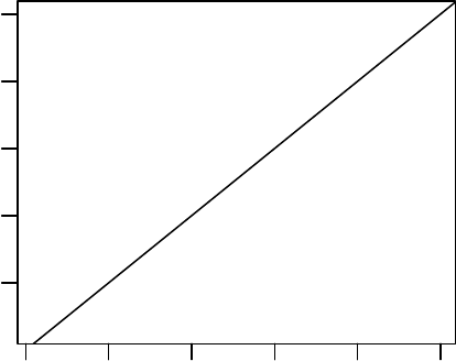
randomized trial, the p-values from the balance tests should follow the line of equality when

compared with the quantiles of the uniform distribution. In Figure 1 we compare the two-sample

p-values for all 35 covariates in the entire number match with near-ﬁne balance to the quantiles

of the uniform distribution. We ﬁnd that the two-sample p-values tend to fall above the line

of equality, which indicates that the match produced greater balance than if we had assigned

the students to treatment or control at random. Of course, randomization would also tend

to balance unobserved covariates, which matching cannot do. However, this implies that any

additional reduction of bias provided by a pair match is probably unnecessary.

●

● ●

●

●●

●

●● ●●

0.0 0.2 0.4 0.6 0.8 1.0

0.2 0.4 0.6 0.8 1.0

Uniform Distribution

Sorted P−values

Figure 1: The quantile-quantile plot compares the 35 two-sample p-values from the match based

on the entire number and a near-ﬁne balance constraint with the uniform distribution. We expect

p-values from a randomized experiment to fall along the line of equality. Balance on observed

covariates does not imply balance on unobserved covariates.

We now compare the variable-ratio match with near-ﬁne balance to two matches possible with

existing algorithms. We denote these two more conventional matches ˛

and ˛

. Both ˛

and ˛

are variable-ratio matches based on minimizing the robust Mahalanobis distances with a

caliper on the propensity score. Neither has any ﬁne or near-ﬁne balance constraints. In ˛

, we

●

0.0 0.2 0.4 0.6 0.8

Absolute Standardized Difference

Unmatched

Pair Match

Variable Ratio

Matching

Entire Matching

With Near−Fine Balance

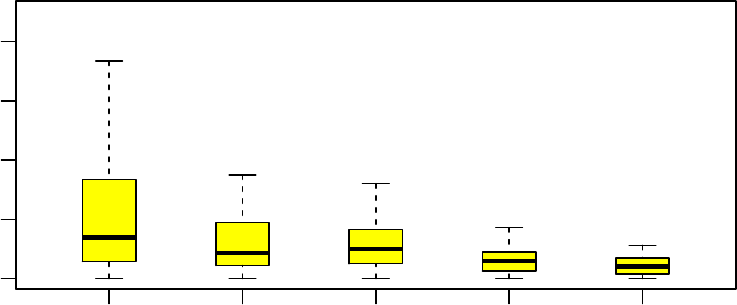
Figure 2: The distribution of absolute standardized diﬀerences for the four matches and the

unmatched data.

implement variable-ratio matching using the entire number. In ˛

, we implement a variable-ratio

match using the optmatch library [16]. In the statistical package R, the fullmatch function in

the optmatch library can be used to create an optimal match with a variable control:treatment

ratio based on a minimum-cost ﬂow algorithm.

These additional matches allow us to compare the match with a variable control:treatment ratio

and a ﬁne balance constraint to two matches that omit ﬁne balance but use a variable con-

trol:treatment ratio. However, the match based on the entire number removes the same ﬁve

treated units that did not meet our common support constraint. The variable ratio match based

on network ﬂows using the fullmatch function includes all observations. Speciﬁcally under this

comparison, we can isolate whether removing observations oﬀ the common support has a large

eﬀect on imbalances.

First, we describe ˛

. Initially we used ˇ D 10 as the maximum number of controls per treated.

However, this resulted in many small strata (4 of the 10 strata produced had fewer than 20

subjects total) in which match quality was often poor. For example, in the stratum with entire

number 9 there were exactly 9 controls and one treated subject. This meant all the controls

were included in the match, even though the treated subject had used drugs in the past 30 days

and only one of the controls had. To avoid such imbalances we decided to reduce the value

of ˇ from 10 to 5. The resulting match used 13 fewer controls (202 total instead of 215) but

had far fewer small strata and allowed better-quality matches on average within each stratum.

Table 4 contains a summary of balance statistics with full results reported in the supplementary

materials. The ˛

match is a major improvement over the pair match. For this match, all of the

standardized diﬀerences were smaller in magnitude than 0.2 and only ﬁve were larger than 0.1.

With this match, we also removed 5 treated units due to a lack of common support. While the

match is a clear improvement over the pair match, the ﬁne balance constraints are useful.

If we do not enforce the ﬁne balance constraint two of the nearly ﬁne balance categories have

standardized diﬀerences that exceed 0.10.

Next, we describe the ˛

match. Again Table 4 provides a brief summary of the results with full

results reported in the supplementary materials. The ˛

match used all 121 treated observations

which produced an eﬀective sample size of 160 pairs. That is, variable-ratio matching based on

the fullmatch function does not remove observations when there is a lack of common support.

Including the additional 5 treated units comes at a considerable cost in terms of balance. In

the ˛

match, 13 covariates still have standardized diﬀerences above 0.10 just as in the pair

match. Without the ﬁne balance constraint for this match balance suﬀers, as two of the nearly

ﬁne balanced categories have standardized diﬀerences that exceed 0.20 and 0.50. We altered the

match to allow for up to 10 controls for each treated unit. This matched produced a much

wider variety of matched strata, and balance that is more comparable to the ˛

match.

Figure 2 provides a ﬁnal comparison of every match and the unmatched data. For each match,

we plot the distribution of absolute standardized diﬀerences. The results follow what theory

suggest. Both the pair match and the match with a variable control:treated ratio use the entire

sample. Therefore, the eﬀective sample size—deﬁned in the ﬁrst part of this section—for the

pair match was 121 matched pairs, and the match with a variable control:treated ratio had an

eﬀective sample size of 160 matched pairs. The lack of common support contributes to the poor

performance of both of these matches, however, we see that the pair match removes more bias.

The entire number match without a near-ﬁne balance constraint drops ﬁve treated observations

which produces a substantial reduction in overt bias. Finally once we add the near-ﬁne balance

constraint, we observe additional bias reduction targeted at an interaction of two speciﬁc nominal

covariates. The eﬀective same size for both matches that use the entire number is 134.5 matched

pairs. As such, we make more eﬀective use of the sample while also removing as much overt bias

as would be expected from a randomized trial.

Generally, we see that to improve on the initial pair match and produce the smallest set of

imbalances using the largest possible number of control units required three separate matching

strategies. First, we implemented a variable-ratio match using the entire number. We also

enforced ﬁne balance constraints and removed ﬁve observations that lacked common support.

This ﬁnal comparison, however, demonstrates that while the common support trimming was

necessary, so too were the near-ﬁne balance constraints.

5 Summary

By using the entire number, one can construct a ﬁne or near-ﬁnely balanced example with a vari-

able control:treatment ratio. In the PHE example, we produce near-ﬁne balance on an interaction

of two nominal covariates while using a variable control:treatment ratio. Using both a variable

control:treatment ratio and a near-ﬁne balance constraint allows us to remove overt biases while

increasing eﬃciency. While it should be possible to remove additional bias using a pair match

with a ﬁne balance constraint, that match will necessarily use fewer controls. Moreover, our ﬁnal

match produced standardized diﬀerences such that the amount of overt bias is less than we would

expect if units had been assigned to treatment and control via randomization.

References

1. Sloane, BC, Zimmer, CG. The power of peer health education. Journal of American College

Health 1993; 41(6):241–245.

2. White, S, Park, YS, Israel, T, Cordero, ED. Longitudinal evaluation of peer health education

on a college campus: Impact on health behaviors. Journal of American College Health 2009;

57(5):497–506.

3. Dunn, L, Ross, B, Caines, T, Howorth, P. A school-based hiv/aids prevention education

program: outcomes of peer-led versus community health nurse-led interventions. Canadian

Journal of Human Sexuality 1998; 7(4):339–345.

4. Forrest, S, Strange, V, Oakley, A. A comparison of students’ evaluations of a peer-delivered

sex education programme and teacher-led provision. Sex Education: Sexuality, Society and

Learning 2002; 2(3):195–214.

5. Kim, CR, Free, C. Recent evaluations of the peer-led approach in adolescent sexual health

education: A systematic review. Perspectives on sexual and reproductive health 2008;

40(3):144–151.

6. Cochran, WG, Chambers, SP. The planning of observational studies of human populations.

Journal of Royal Statistical Society, Series A 1965; 128(2):234–265.

7. Rubin, DB. Estimating causal eﬀects of treatments in randomized and nonrandomized studies.

Journal of Educational Psychology 1974; 6(5):688–701.

8. Rosenbaum, PR, Rubin, DB. The central role of propensity scores in observational studies

for causal eﬀects. Biometrika 1983; 76(1):41–55.

9. Rosenbaum, PR. Optimal matching for observational studies. Journal of the American

Statistical Association 1989; 84(4):1024–1032.

10. Ming, K, Rosenbaum, PR. Substantial gains in bias reduction from matching with a variable

number of controls. Biometrics 2000; 56(1):118–124.

11. Hansen, BB. Full matching in an observational study of coaching for the sat. Journal of the

American Statistical Association 2004; 99(467):609–618.

12. Zubizarreta, JR. Using mixed integer programming for matching in an observational study

of kidney failure after surgery. Journal of the American Statistical Association 2012;

107(500):1360–1371.

13. Rubin, DB. The design versus the analysis of observational studies for causal eﬀects: parallels

with the design of randomized trials. Statistics in medicine 2007; 26(1):20–36.

14. Rubin, DB. For objective causal inference, design trumps analysis. The Annals of Applied

Statistics 2008; 2(3):808–840.

15. Rosenbaum, PR. Design of Observational Studies. Springer-Verlag, New York, 2010.

16. Hansen, BB. Optmatch. R News 2007; 7(2):18–24.

17. Rosenbaum, PR, Ross, RN, Silber, JH. Mimimum distance matched sampling with ﬁne

balance in an observational study of treatmetnt for ovarian cancer. Journal of the American

Statistical Association 2007; 102(477):75–83.

18. Yang, D, Small, DS, Silber, JH, Rosenbaum, PR. Optimal matching with minimal deviation

from ﬁne balance in a study of obesity and surgical outcomes. Biometrics 2012; 68(2):628–

636.

19. Rosenbaum, PR. A characterization of optimal designs for observational studies. Journal of

the Royal Statistical Society. Series B (Methodological) 1991; :597–610.

20. Bertsekas, DP. A new algorithm for the assignment problem. Mathematical Programming

1981; 21(1):152–171.

21. Iacus, SM, King, G, Porro, G. Causal inference without balance checking: Coarsened exact

matching. Political Analysis 2011; 20(1):1–24.

22. Diamond, A, Sekhon, JS. Genetic matching for estimating causal eﬀects: A general multi-

variate matching method for achieving balance in observational studies. Review of Economics

and Statistics 2013; 95(3):932–945.

23. Yoon, FB. New Methods for the Design and Analysis of Observational Studies. Ph.D. thesis,

University of Pennsylvania, 2009.

24. Ming, K, Rosenbaum, PR. A note on optimal matching with variable controls using the

assignment algorithm. Journal of Computational and Graphical Statistics 2001; 10(3):455–

463.

25. Stuart, EA. Matching methods for causal inference: A review and a look forward. Statistical

Science 2010; 25(1):1–21.

26. Stuart, EA, Green, KM. Using full matching to estimate causal eﬀects in nonexperimental

studies: examining the relationship between adolescent marijuana use and adult outcomes.

Developmental Psychology 2008; 44(2):395–406.

27. Rosenbaum, PR, Rubin, DB. Reducing bias in observational studies using subclassiﬁcation on

the propensity score. Journal of the American Statistical Association 1984; 79(387):516–524.

28. Crump, RK, Hotz, VJ, Imbens, GW, Mitnik, OA. Dealing with limited overlap in estimation

of average treatment eﬀects. Biometrika 2009; 96(1):187–199.

29. Rosenbaum, PR. Optimal matching of an optimally chosen subset in observational studies.

Journal of Computational and Graphical Statistics 2012; 21(1):57–71.

30. Dehejia, R, Wahba, S. Causal eﬀects in non-experimental studies: Re-evaluating the

evalulation of training programs. Journal of the American Statistical Association 1999;

94(448):1053–1062.

31. Traskin, M, Small, DS. Deﬁning the study population for an observational study to ensure

suﬃcient overlap: a tree approach. Statistics in Biosciences 2011; 3(1):94–118.

32. Team, RDC. R: A Language and Environment for Statistical Computing. R Foundation for

Statistical Computing, Vienna, Austria, 2014.