
OPERATING SYSTEM
Lecture Notes
On
Prepared by,
A.SANDEEP.
ASSISTANT PROFESSOR.
CSE

Page 1
OPERATING
SYSTEM
LECTURE NOTES
Page 2
OPERATING SYSTEM
Lecture Notes
Lecture #1
What is an Operating System?
A program that acts as an intermediary between a user of a computer and the computer hardware.
An operating System is a collection of system programs that together control the operations of a computer
system.
Some examples of operating systems are UNIX, Mach, MS-DOS, MS-Windows, Windows/NT, Chicago, OS/2,
MacOS, VMS, MVS, and VM.
Operating system goals:
Execute user programs and make solving user problems easier.
Make the computer system convenient to use.
Use the computer hardware in an efficient manner.
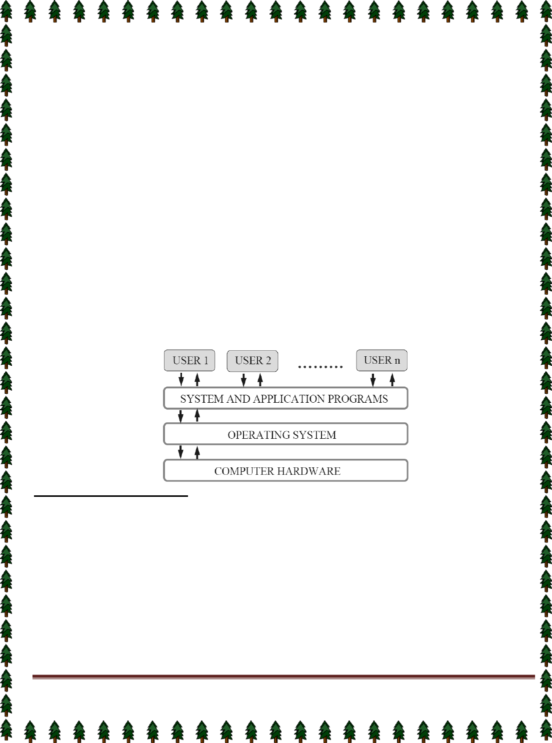
Computer System Components
1.
Hardware – provides basic computing resources (CPU, memory, I/O devices).
2.
Operating system – controls and coordinates the use of the hardware among the various application
programs for the various users.
3.
Applications programs – Define the ways in which the system resources are used to solve the computing
problems of the users (compilers, database systems, video games, business programs).
4.
Users (people, machines, other computers).
Abstract View of System Components
Operating System Definitions
Resource allocator – manages and allocates resources.
Control program – controls the execution of user programs and operations of I/O devices .
Kernel – The one program running at all times (all else being application programs).
Components of OS: OS has two parts. (1)Kernel.(2)Shell.
(1)
Kernel is an active part of an OS i.e., it is the part of OS running at all times. It is a programs which
can interact with the hardware. Ex: Device driver, dll files, system files etc.
(2)
Shell is called as the command interpreter. It is a set of programs used to interact with the application
programs. It is responsible for execution of instructions given to OS (called commands).
Operating systems can be explored from two viewpoints: the user and the system.
User View: From the user’s point view, the OS is designed for one user to monopolize its resources, to
maximize the work that the user is performing and for ease of use.
System View: From the computer's point of view, an operating system is a control program that manages the
execution of user programs to prevent errors and improper use of the computer. It is concerned with the
operation and control of I/O devices.

Page 3
Lecture #2
Functions of Operating System:
Process Management
A process is a program in execution. A process needs certain resources, including CPU time, memory,
files, and I/O devices, to accomplish its task.
The operating system is responsible for the following activities in connection with process management.
✦ Process creation and deletion.
✦ process suspension and resumption.
✦ Provision of mechanisms for:
process synchronization
process communication
Main-Memory Management
Memory is a large array of words or bytes, each with its own address. It is a repository of quickly
accessible data shared by the CPU and I/O devices.
Main memory is a volatile storage device. It loses its contents in the case of system failure.
The operating system is responsible for the following activities in connections with memory management:
Keep track of which parts of memory are currently being used and by whom.
Decide which processes to load when memory space becomes available.
Allocate and de-allocate memory space as needed.
File Management
A file is a collection of related information defined by its creator. Commonly, files represent programs
(both source and object forms) and data.
The operating system is responsible for the following activities in connections with file management:
✦ File creation and deletion.
✦ Directory creation and deletion.
✦ Support of primitives for manipulating files and directories.
✦ Mapping files onto secondary storage.
✦ File backup on stable (nonvolatile) storage media.
I/O System Management
The I/O system consists of:
✦ A buffer-caching system
✦ A general device-driver interface
✦ Drivers for specific hardware devices
Secondary-Storage Management
Since main memory (primary storage) is volatile and too small to accommodate all data and programs
permanently, the computer system must provide secondary storage to back up main memory.
Most modern computer systems use disks as the principle on-line storage medium, for both programs and data.
The operating system is responsible for the following activities in connection with disk management:
✦ Free space management
✦ Storage allocation
✦ Disk scheduling
Networking (Distributed Systems)
A distributed system is a collection processors that do not share memory or a clock. Each processor has
its own local memory.
The processors in the system are connected through a communication network.
Communication takes place using a protocol.
A distributed system provides user access to various system resources.
Access to a shared resource allows:
✦ Computation speed-up

Page 4
✦ Increased data availability
✦ Enhanced reliability
Protection System
Protection refers to a mechanism for controlling access by programs, processes, or users to both
system and user resources.
The protection mechanism must:
✦ distinguish between authorized and unauthorized usage.
✦ specify the controls to be imposed.
✦ provide a means of enforcement.
Command-Interpreter System
Many commands are given to the operating system by control statements which deal with:
✦ process creation and management
✦ I/O handling
✦ secondary-storage management
✦ main-memory management
✦ file-system access
✦ protection
✦ networking
The program that reads and interprets control statements is called variously:
✦ command-line interpreter
✦ shell (in UNIX)
Its function is to get and execute the next command statement.
Operating-System Structures
System Components
Operating System Services
System Calls
System Programs
System Structure
Virtual Machines
System Design and Implementation
System Generation
Common System Components
Process Management
Main Memory Management
File Management
I/O System Management
Secondary Management
Networking
Protection System
Command-Interpreter System

Page 5
Lecture #3
Evolution of OS:
1.
Mainframe Systems
Reduce setup time by batching similar jobs Automatic job sequencing – automatically transfers control from one
job to another. First rudimentary
operating system. Resident monitor
initial control in monitor
control transfers to job
when job completes control transfers pack to monitor
2.
Batch Processing Operating System:
This type of OS accepts more than one jobs and these jobs are batched/ grouped together according to their
similar requirements. This is done by computer operator. Whenever the computer becomes available, the
batched jobs are sent for execution and gradually the output is sent back to the user.
It allowed only one program at a time.
This OS is responsible for scheduling the jobs according to priority and the resource required.
3.
Multiprogramming Operating System:
This type of OS is used to execute more than one jobs simultaneously by a single processor. it increases CPU
utilization by organizing jobs so that the CPU always has one job to execute.
The concept of multiprogramming is described as follows:
All the jobs that enter the system are stored in the job pool( in disc). The operating system loads a set
of jobs from job pool into main memory and begins to execute.
During execution, the job may have to wait for some task, such as an I/O operation, to complete. In
a multiprogramming system, the operating system simply switches to another job and executes.
When that job needs to wait, the CPU is switched to
another
job, and so on.
When the first job finishes waiting and it gets the CPU back.
As long as at least one job needs to execute, the CPU is never idle.
Multiprogramming operating systems use the mechanism of job scheduling and CPU scheduling.
3. Time-Sharing/multitasking Operating Systems
Time sharing (or multitasking) OS is a logical extension of multiprogramming. It provides extra facilities such as:
Faster switching between multiple jobs to make processing faster.
Allows multiple users to share computer system simultaneously.
The users can interact with each job while it is running.
These systems use a concept of virtual memory for effective utilization of memory space. Hence, in this OS, no
jobs are discarded. Each one is executed using virtual memory concept. It uses CPU scheduling, memory
management, disc management and security management. Examples: CTSS, MULTICS, CAL, UNIX etc.
4. Multiprocessor Operating Systems
Multiprocessor operating systems are also known as parallel OS or tightly coupled OS. Such operating
systems have more than one processor in close communication that sharing the computer bus, the clock and
sometimes memory and peripheral devices. It executes multiple jobs at same time and makes the processing
faster.
Multiprocessor systems have three main advantages:
Increased throughput: By increasing the number of processors, the system performs more work in less time.
The speed-up ratio with
N
processors is less than
N
.
Economy of scale: Multiprocessor systems can save more money than multiple single-processor systems,
because they can share peripherals, mass storage, and power supplies.
Increased reliability: If one processor fails to done its task, then each of the remaining processors must pick
up a share of the work of the failed processor. The failure of one processor will not halt the system, only
slow it down.
The ability to continue providing service proportional to the level of surviving hardware is called graceful
degradation. Systems designed for graceful degradation are called fault tolerant.

Page 6
The multiprocessor operating systems are classified into two categories:
1.
Symmetric multiprocessing system
2.
Asymmetric multiprocessing system
In symmetric multiprocessing system, each processor runs an identical copy of the operating system, and
these copies communicate with one another as needed.
In asymmetric multiprocessing system, a processor is called master processor that controls other processors
called slave processor. Thus, it establishes master-slave relationship. The master processor schedules the jobs
and manages the memory for entire system.
5. Distributed Operating Systems
In distributed system, the different machines are connected in a network and each machine has its own
processor and own local memory.
In this system, the operating systems on all the machines work together to manage the collective network
resource.
It can be classified into two categories:
1.
Client-Server systems
2.
Peer-to-Peer systems
Advantages of distributed systems.
Resources Sharing
Computation speed up – load sharing
Reliability
Communications
Requires networking infrastructure.
Local area networks (LAN) or Wide area networks (WAN)
.
6. Desktop Systems/Personal Computer Systems
The PC operating system is designed for maximizing user convenience and responsiveness. This system is
neither multi-user nor multitasking.
These systems include PCs running Microsoft Windows and the Apple Macintosh. The MS-DOS operating
system from Microsoft has been superseded by multiple flavors of Microsoft Windows and IBM has
upgraded MS-DOS to the OS/2 multitasking system.
The Apple Macintosh operating system has been ported to more advanced hardware, and now includes new
features such as virtual memory and multitasking.
7. Real-Time Operating Systems (RTOS)
A real-time operating system (RTOS) is a multitasking operating system intended for applications with fixed
deadlines (real-time computing). Such applications include some small embedded systems, automobile
engine controllers, industrial robots, spacecraft, industrial control, and some large-scale computing systems.
The real time operating system can be classified into two categories:
1.
hard real time system and 2. soft real time system.
A hard real-time system guarantees that critical tasks be completed on time. This goal requires that all
delays in the system be bounded, from the retrieval of stored data to the time that it takes the operating
system to finish any request made of it. Such time constraints dictate the facilities that are available in hard real-
time systems.
A soft real-time system is a less restrictive type of real-time system. Here, a critical real-time task gets
priority over other tasks and retains that priority until it completes. Soft real time system can be mixed with
other types of systems. Due to less restriction, they are risky to use for industrial control and robotics.

Page 7
Operating System Services
Lecture #4
Following are the five services provided by operating systems to the convenience of the users.
1.
Program Execution
The purpose of computer systems is to allow the user to execute programs. So the operating system
provides an environment where the user can conveniently run programs. Running a program involves the
allocating and deallocating memory, CPU scheduling in case of multiprocessing.
2.
I/O Operations
Each program requires an input and produces output. This involves the use of I/O. So the operating
systems are providing I/O makes it convenient for the users to run programs.
3.
File System Manipulation
The output of a program may need to be written into new files or input taken from some files. The
operating system provides this service.
4.
Communications
The processes need to communicate with each other to exchange information during execution. It may
be between processes running on the same computer or running on the different computers. Communications
can be occur in two ways: (i) shared memory or (ii) message passing
5.
Error Detection
An error is one part of the system may cause malfunctioning of the complete system. To avoid such a
situation operating system constantly monitors the system for detecting the errors. This relieves the user of the
worry of errors propagating to various part of the system and causing malfunctioning.
Following are the three services provided by operating systems for ensuring the efficient operation of
the system itself.
1.
Resource allocation
When multiple users are logged on the system or multiple jobs are running at the same time, resources
must be allocated to each of them. Many different types of resources are managed by the operating system.
2.
Accounting
The operating systems keep track of which users use how many and which kinds of computer resources.
This record keeping may be used for accounting (so that users can be billed) or simply for accumulating usage
statistics.
3.
Protection
When several disjointed processes execute concurrently, it should not be possible for one process to
interfere with the others, or with the operating system itself. Protection involves ensuring that all access to
system resources is controlled. Security of the system from outsiders is also important. Such security starts with
each user having to authenticate him to the system, usually by means of a password, to be allowed access to the
resources.
System Call:
System calls provide an interface between the process and the operating system.
System calls allow user-level processes to request some services from the operating system which process
itself is not allowed to do.
For example, for I/O a process involves a system call telling the operating system to read or write particular
area and this request is satisfied by the operating system.
The following different types of system calls provided by an operating system:
Process control
end, abort
load, execute
create process, terminate process
get process attributes, set process attributes
wait for time
wait event, signal event
allocate and free memory
Page 8
File management
create file, delete file
open, close
read, write, reposition
get file attributes, set file attributes
Device management
request device, release device
read, write, reposition
get device attributes, set device attributes
logically attach or detach devices
Information maintenance
get time or date, set time or date
get system data, set system data
get process, file, or device attributes
set process, file, or device attributes
Communications
create, delete communication connection
send, receive messages
transfer status information
attach or detach remote devices
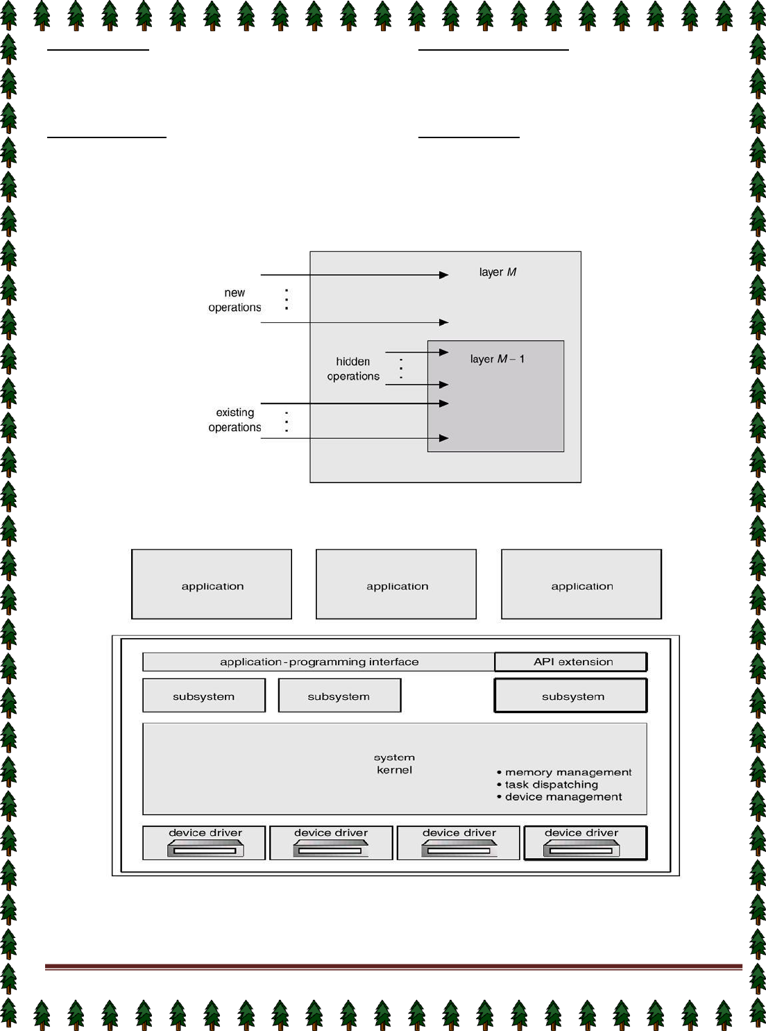
An Operating System Layer
OS/2 Layer Structure
Microkernel System Structure
Moves as much from the kernel into “user” space.
Communication takes place between user modules using message passing.
Benefits:
Page 9
easier to extend a microkernel
easier to port the operating system to new architectures
more reliable (less code is running in kernel mode)
more secure
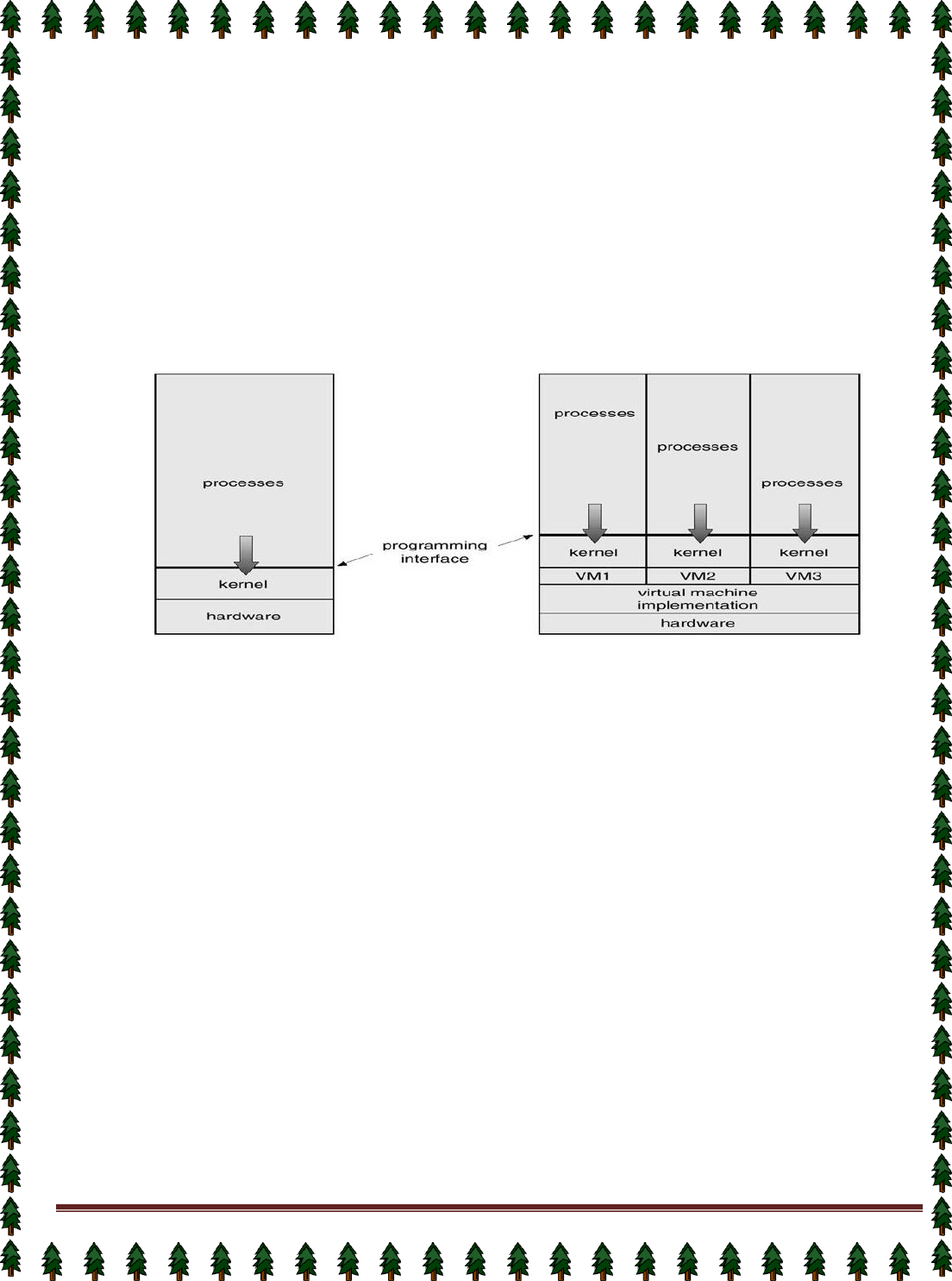
Virtual Machines
A virtual machine takes the layered approach to its logical conclusion. It treats hardware and the
operating system kernel as though they were all hardware.
A virtual machine provides an interface identical to the underlying bare hardware.
The operating system creates the illusion of multiple processes, each executing on its own processor
with its own (virtual) memory.
The resources of the physical computer are shared to create the virtual machines.
✦ CPU scheduling can create the appearance that users have their own processor.
✦ Spooling and a file system can provide virtual card readers and virtual line printers.
✦ A normal user time-sharing terminal serves as the virtual machine operator’s console.
System Models
Non-virtual Machine Virtual Machine
Advantages/Disadvantages of Virtual Machines
The virtual-machine concept provides complete protection of system resources since each virtual
machine is isolated from all other virtual machines. This isolation, however, permits no direct sharing of
resources.
A virtual-machine system is a perfect vehicle for operating-systems research and development. System
development is done on the virtual machine, instead of on a physical machine and so does not disrupt
normal system operation.
The virtual machine concept is difficult to implement due to the effort required to provide an exact
duplicate to the underlying machine.
System Generation (SYSGEN)
Operating systems are designed to run on any of a class of machines at a variety of sites with a variety
of peripheral configurations. The system must then be configured or generated for each specific computer site, a
process sometimes known as system generation (SYSGEN).
SYSGEN program obtains information concerning the specific configuration of the hardware system.
To generate a system, we use a special program. The SYSGEN program reads from a given file, or asks the
operator of the system for information concerning the specific configuration of the hardware system, or probes
the hardware directly to determine what components are there.
The following kinds of information must be determined.
What CPU will be used? What options (extended instruction sets, floating point arithmetic, and so on) are
installed? For multiple-CPU systems, each CPU must be described.
How much memory is available? Some systems will determine this value themselves by referencing memory
location after memory location until an "illegal address" fault is generated. This procedure defines the final legal
address and hence the amount of available memory.
What devices are available? The system will need to know how to address each device (the device number), the
device interrupt number, the device's type and model, and any special device characteristics.
Page 10
What operating-system options are desired, or what parameter values are to be used? These options or values
might include how many buffers of which sizes should be used, what type of CPU-scheduling algorithm is
desired, what the maximum number of processes to be supported is.
Booting –The procedure of starting a computer by loading the kernel is known as booting the system. Most
computer systems have a small piece of code, stored in ROM, known as the bootstrap program or bootstrap
loader. This code is able to locate the kernel, load it into main memory, and start its execution. Some computer
systems, such as PCs, use a two-step process in which a simple bootstrap loader fetches a more complex boot
program from disk, which in turn loads the kernel.
Lecture #5
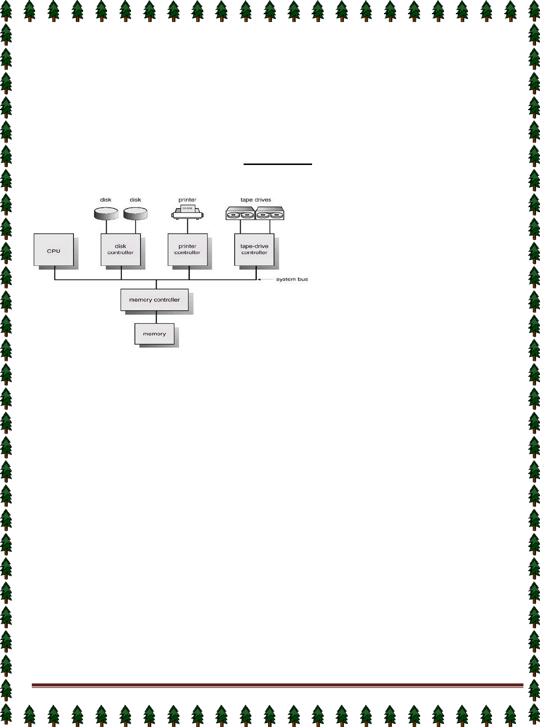
Computer-System Architecture
Computer-System Operation
I/O devices and the CPU can execute concurrently.
Each device controller is in charge of a particular device type.
Each device controller has a local buffer.
CPU moves data from/to main memory to/from local buffers
I/O is from the device to local buffer of controller.
Device controller informs CPU that it has finished its operation by causing an interrupt.
Common Functions of Interrupts
Interrupt transfers control to the interrupt service routine generally, through the interrupt vector, which
contains the addresses of all the service routines.
Interrupt architecture must save the address of the interrupted instruction.
Incoming interrupts are disabled while another interrupt is being processed to prevent a lost interrupt.
A trap is a software-generated interrupt caused either by an error or a user request.
An operating system is interrupt driven.
Interrupt Handling
The operating system preserves the state of the CPU by storing registers and the program counter.
Determines which type of interrupt has occurred: polling, vectored interrupt system
Separate segments of code determine what action should be taken for each type of interrupt
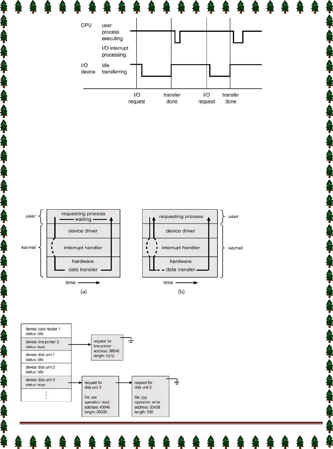
Interrupt Time Line For a Single Process Doing Output
Page 11
I/O Structure
After I/O starts, control returns to user program only upon I/O completion.
✦ Wait instruction idles the CPU until the next interrupt
✦ Wait loop (contention for memory access).
✦ At most one I/O request is outstanding at a time, no simultaneous I/O processing.
After I/O starts, control returns to user program without waiting for I/O completion.
✦ System call – request to the operating system to allow user to wait for I/O completion.
✦ Device-status table contains entry for each I/O device indicating its type, address, and state.
✦ Operating system indexes into I/O device table to determine device status and to modify table entry to include
interrupt.
Two I/O Methods
Synchronous Asynchronous
Device-Status Table

Page 12
Direct Memory Access Structure
Used for high-speed I/O devices able to transmit information at close to memory speeds.
Device controller transfers blocks of data from buffer storage directly to main memory without CPU
intervention.
Only on interrupt is generated per block, rather than the one interrupt per byte.
Storage Structure
Main memory – only large storage media that the CPU can access directly.
Secondary storage – extension of main memory that provides large nonvolatile storage capacity.
Magnetic disks – rigid metal or glass platters covered with magnetic recording material
✦ Disk surface is logically divided into tracks, which are subdivided into sectors.
✦ The disk controller determines the logical interaction between the device and the computer.
Storage Hierarchy
Storage systems organized in hierarchy.
✦ Speed
✦ Cost
✦ Volatility
Caching – copying information into faster storage system; main memory can be viewed as a last cache for
secondary storage.
Use of high-speed memory to hold recently-accessed data.
Requires a cache management policy.
Caching introduces another level in storage hierarchy.
This requires data that is simultaneously stored in more than one level to be consistent.
Storage-Device Hierarchy
Hardware Protection
Dual-Mode Operation

Page 13
I/O Protection
Memory Protection
CPU Protection
Dual-Mode Operation
Sharing system resources requires operating system to ensure that an incorrect program cannot cause
other programs to execute incorrectly.
Provide hardware support to differentiate between at least two modes of operations.
User mode – execution done on behalf of a user.
Monitor mode (also kernel mode or system mode) – execution done on behalf of operating system.
Mode bit added to computer hardware to indicate the current mode: monitor (0) or user (1).
When an interrupt or fault occurs hardware switches to Privileged instructions can be issued only in
monitor mode.
monitor user ,Interrupt/fault ,set user mode
I/O Protection
All I/O instructions are privileged instructions.
Must ensure that a user program could never gain control of the computer in monitor mode (I.e.a
user program that, as part of its execution, stores a new address in the
interrupt vector).
Memory Protection
Must provide memory protection at least for the interrupt vector and the interrupt service routines.
In order to have memory protection, add two registers that determine the range of legal addresses a
program may access:
✦ Base register – holds the smallest legal physical memory address.
✦ Limit register – contains the size of the range
Memory outside the defined range is protected.
Hardware Protection
When executing in monitor mode, the operating system has unrestricted access to both monitor and
user’s memory.
The load instructions for the base and limit registers are privileged instructions.
CPU Protection
Timer – interrupts computer after specified period to ensure operating system maintains control.
✦ Timer is decremented every clock tick.
✦ When timer reaches the value 0, an interrupt occurs.
Timer commonly used to implement time sharing.
Time also used to compute the current time.
Load-timer is a privileged instruction.
Page 14
Process Concept
Lecture #6(UNIT-II)
Informally, a process is a program in execution. A process is more than the program code, which is
sometimes known as the text section. It also includes the current activity, as represented by the value of
the program counter and the contents of the processor's registers. In addition, a process generally
includes the process stack, which contains temporary data (such as method parameters, return
addresses, and local variables), and a data section, which contains global variables.
An operating system executes a variety of programs:
✦ Batch system – jobs
✦ Time-shared systems – user programs or tasks
Process – a program in execution; process execution must progress in sequential fashion.
A process includes: program counter , stack, data section
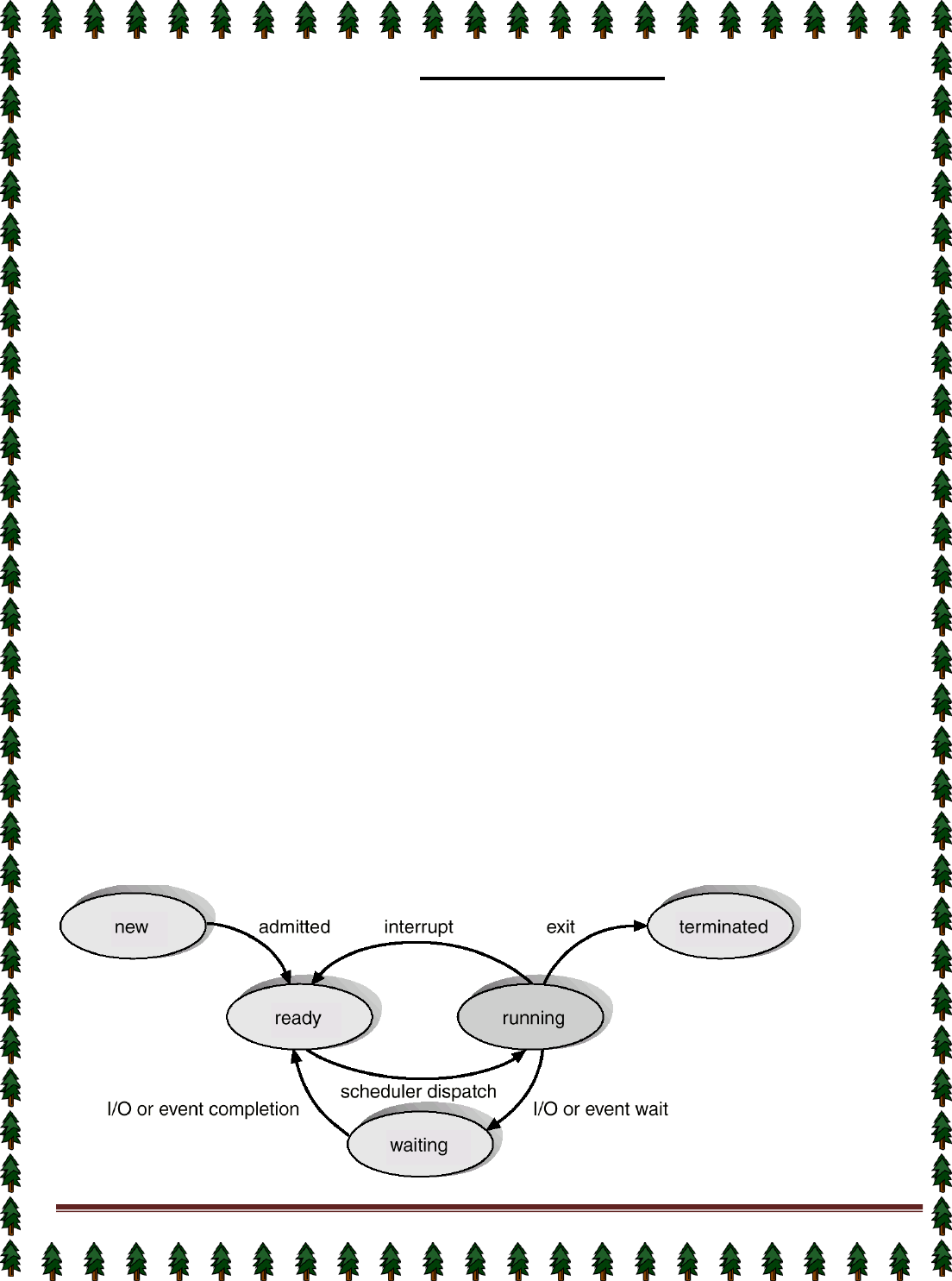
Process State
As a process executes, it changes state
New State: The process is being created.
Running State: A process is said to be running if it has the CPU, that is, process actually using the CPU at
that particular instant.
Blocked (or waiting) State: A process is said to be blocked if it is waiting for some event to happen such that
as an I/O completion before it can proceed. Note that a process is unable to run until some external event
happens.
Ready State: A process is said to be ready if it needs a CPU to execute. A ready state process is runnable
but temporarily stopped running to let another process run.
Terminated state: The process has finished execution.
What is the difference between process and program?
1)
Both are same beast with different name or when this beast is sleeping (not executing) it is called program
and when it is executing becomes process.
2)
Program is a static object whereas a process is a dynamic object.
3)
A program resides in secondary storage whereas a process resides in main memory.
4)
The span time of a program is unlimited but the span time of a process is limited.
5)
A process is an 'active' entity whereas a program is a 'passive' entity.
6)
A program is an algorithm expressed in programming language whereas a process is expressed in assembly
language or machine language.
Diagram of Process State
Page 15
Lecture #7,#8
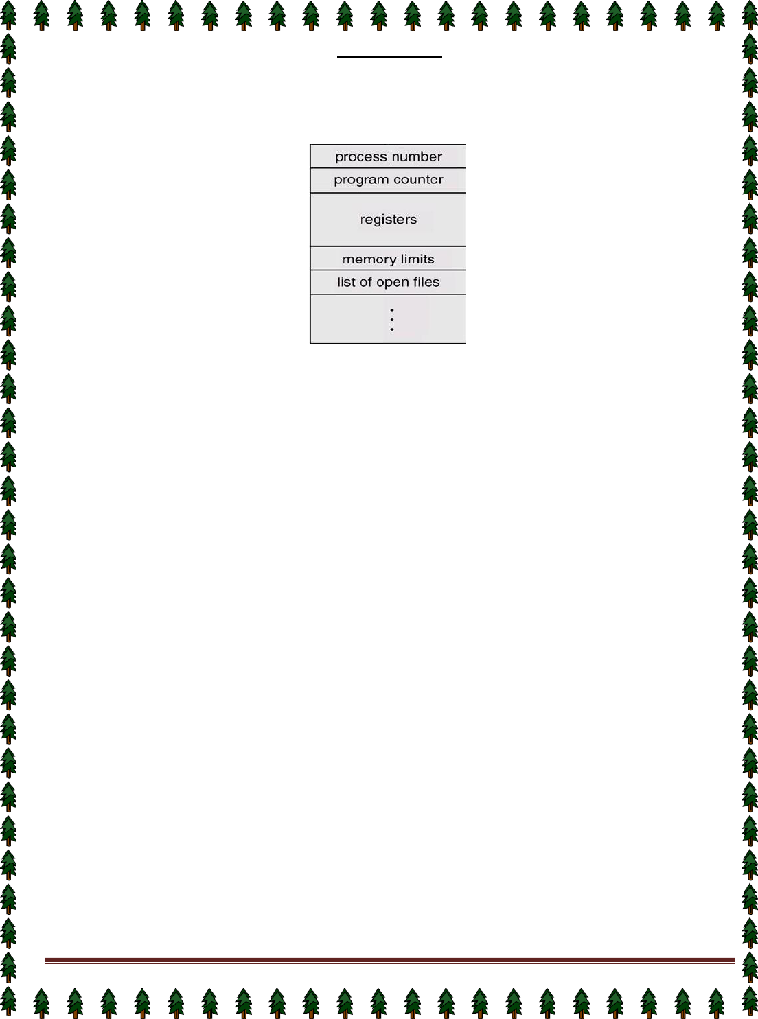
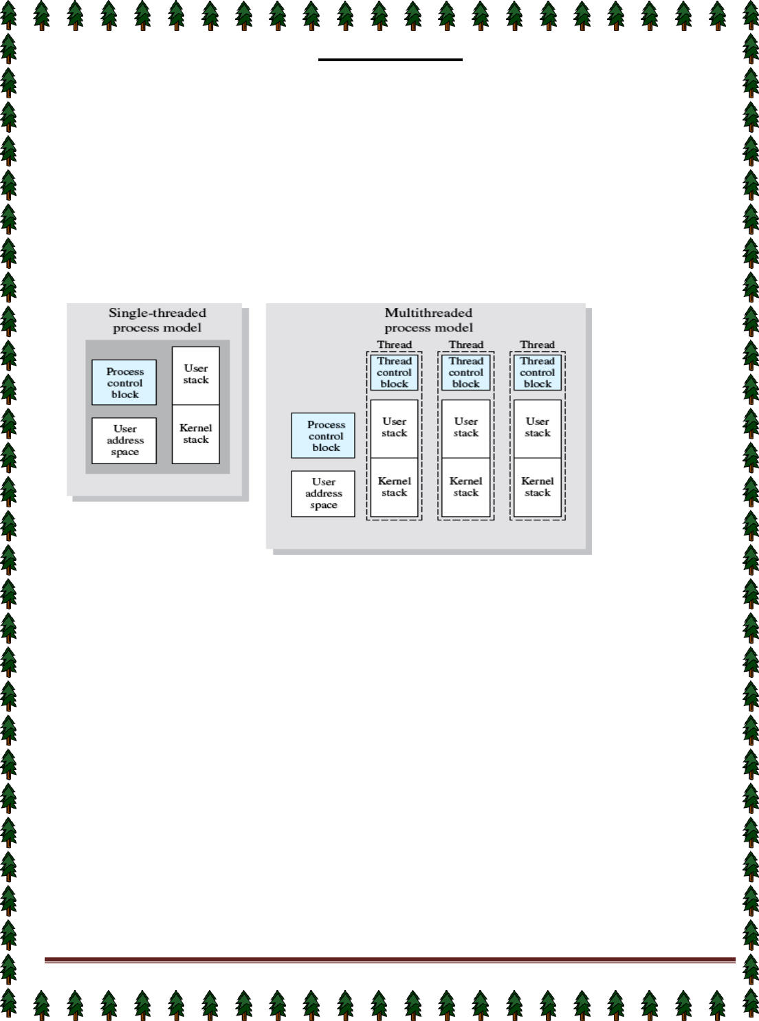
Process Control Block (PCB)
Information associated with each process.
Process state
Program counter
CPU registers
CPU scheduling information
Memory-management information
Accounting information
I/O status information
Process state: The state may be new, ready, running, waiting, halted, and SO on.
Program counter: The counter indicates the address of the next instruction to be executed for this process.
CPU registers: The registers vary in number and type, depending on the computer architecture. They include
accumulators, index registers, stack pointers, and general-purpose registers, plus any condition-code
information. Along with the program counter, this state information must be saved when an interrupt occurs, to
allow the process to be continued correctly afterward.
CPU-scheduling information: This information includes a process priority, pointers to scheduling queues, and
any other scheduling parameters.
Memory-management information: This information may include such information as the value of the base and
limit registers, the page tables, or the segment tables, depending on the memory system used by the operating
system.
Accounting information: This information includes the amount of CPU and real time used, time limits, account
numbers, job or process numbers, and so on.
status information: The information includes the list of I/O devices allocated to this process, a list of open files,
and so on.
The PCB simply serves as the repository for any information that may vary
from process to process.
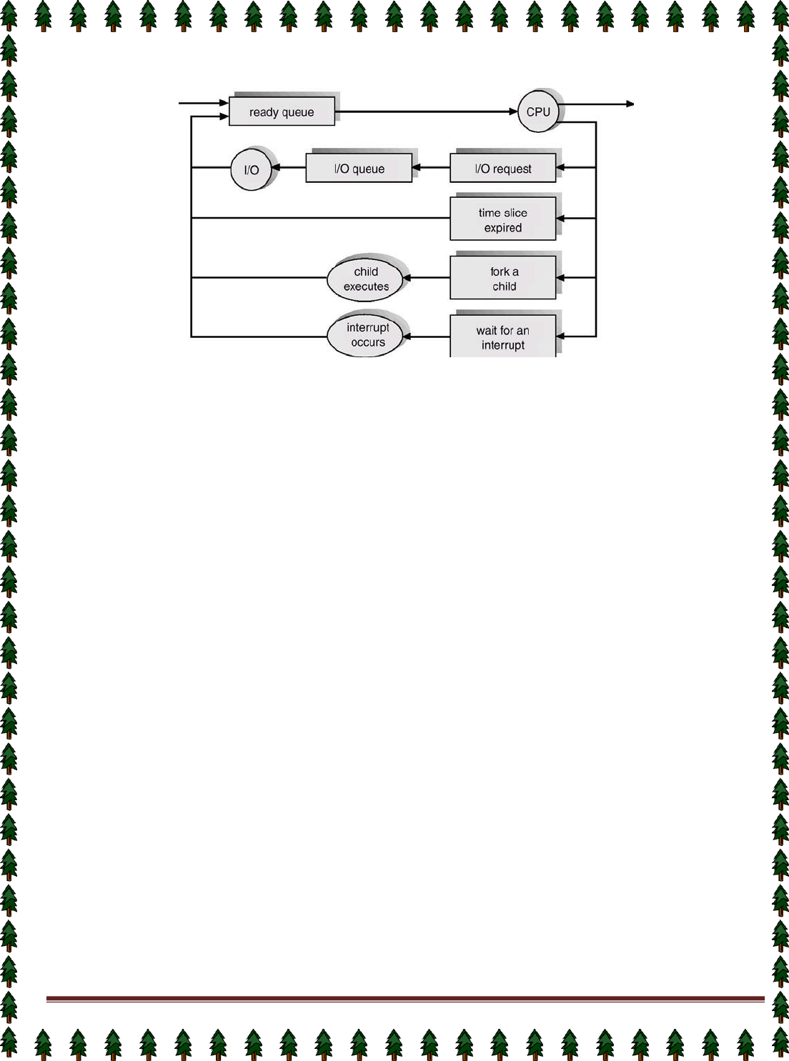
Process Scheduling Queues
Job Queue: This queue consists of all processes in the system; those processes are entered to the system
as new processes.
Ready Queue: This queue consists of the processes that are residing in main memory and are ready and
waiting to execute by CPU. This queue is generally stored as a linked list. A ready-queue header contains
pointers to the first and final PCBs in the list. Each PCB includes a pointer field that points to the next PCB in
the ready queue.
Device Queue: This queue consists of the processes that are waiting for a particular I/O device. Each
device has its own device queue.
Page 16
Representation of Process Scheduling
Schedulers
A scheduler is a decision maker that selects the processes from one scheduling queue to another or
allocates CPU for execution. The Operating System has three types of scheduler:
1.
Long-term scheduler or Job scheduler
2.
Short-term scheduler or CPU scheduler
3.
Medium-term scheduler
Long-term scheduler or Job scheduler
The long-term scheduler or job scheduler selects processes from discs and loads them into main memory for
execution. It executes much less frequently.
It controls the degree of multiprogramming (i.e., the number of processes in memory).
Because of the longer interval between executions, the long-term scheduler can afford to take more time to
select a process for execution.
Short-term scheduler or CPU scheduler
The short-term scheduler or CPU scheduler selects a process from among the processes that are ready to
execute and allocates the CPU.
The short-term scheduler must select a new process for the CPU frequently. A process may execute for only
a few milliseconds before waiting for an I/O request.
Medium-term scheduler
The medium-term scheduler schedules the processes as intermediate level of scheduling
Processes can be described as either:
✦I/O-bound process – spends more time doing I/O than computations, many short CPU bursts.
✦CPU-bound process – spends more time doing computations; few very long CPU bursts.
Context Switch
When CPU switches to another process, the system must save the state of the old process and load the
saved state for the new process.
Context-switch time is overhead; the system does no useful work while switching.

Page 17
Time dependent on hardware support.
Process Creation
Parent process create children processes, which, in turn create other processes, forming a tree of
processes.
Resource sharing:✦ Parent and children share all resources.
✦ Children share subset of parent’s resources.
✦ Parent and child share no resources.
Execution: ✦ Parent and children execute concurrently.
✦ Parent waits until children terminate.
Address space: ✦ Child duplicate of parent.
✦ Child has a program loaded into it.
UNIX examples
✦ fork system call creates new process
✦ exec system call used after a fork to replace the process’ memory space with a new program.
Process Termination
Process executes last statement and asks the operating system to decide it (exit).
✦ Output data from child to parent (via wait).
✦ Process’ resources are deallocated by operating system.
Parent may terminate execution of children processes (abort).
✦ Child has exceeded allocated resources.
✦ Task assigned to child is no longer required.
✦ Parent is exiting.
✔ Operating system does not allow child to continue if its parent terminates.
✔ Cascading termination.
Cooperating Processes
The concurrent processes executing in the operating system may be either independent processes or
cooperating processes. A process is independent if it cannot affect or be affected by the other processes
executing in the system. Clearly, any process that does not share any data (temporary or persistent) with any
other process is independent. On the other hand, a process is cooperating if it can affect or be affected by the
other processes executing in the system. Clearly, any process that shares data with other processes is a
cooperating process.
Advantages of process cooperation
Information sharing: Since several users may be interested in the same piece of information (for instance, a
shared file), we must provide an environment to allow concurrent access to these types of resources.
Computation speedup: If we want a particular task to run faster, we must break it into subtasks, each of which
will be executing in parallel with the others. Such a speedup can be achieved only if the computer has multiple
processing elements (such as CPUS or I/O channels).
Modularity: We may want to construct the system in a modular fashion, dividing the system functions into
separate processes or threads
Convenience: Even an individual user may have many tasks on which to work at one time. For instance, a user
may be editing, printing, and compiling in parallel.
Concurrent execution of cooperating processes requires mechanisms that allow processes to communicate with
one another and to synchronize their actions.
Page 18
Lecture #9,#10,#11,#12
CPU Scheduling
Basic Concepts
Scheduling Criteria
Scheduling Algorithms
Multiple-Processor Scheduling
Real-Time Scheduling
Algorithm Evaluation
Basic Concepts
Maximum CPU utilization obtained with multiprogramming
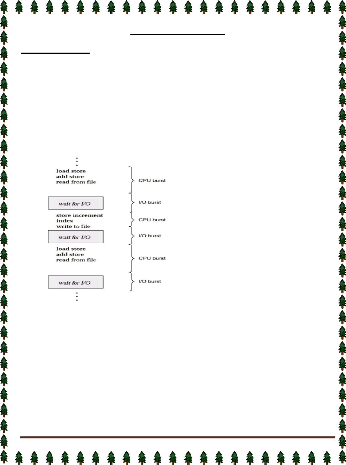
CPU–I/O Burst Cycle – Process execution consists of a cycle of CPU execution and I/O wait.
CPU burst distribution
Alternating Sequence of CPU And I/O Bursts
CPU Scheduler
Selects from among the processes in memory that are ready to execute, and allocates the CPU to one
of them.
CPU scheduling decisions may take place when a process:
1.
Switches from running to waiting state.
2.
Switches from running to ready state.
3.
Switches from waiting to ready.
4.
Terminates.
Scheduling under 1 and 4 is non preemptive.
All other scheduling is preemptive.
Dispatcher
Dispatcher module gives control of the CPU to the process selected by the short-term scheduler; this
involves:
✦ switching context
Page 19
✦ switching to user mode
✦ jumping to the proper location in the user program to restart that program
Dispatch latency – time it takes for the dispatcher to stop one process and start another running.
Scheduling Criteria
CPU utilization – keep the CPU as busy as possible
Throughput – # of processes that complete their execution per time unit
Turnaround time – amount of time to execute a particular process
Waiting time – amount of time a process has been waiting in the ready queue
Response time – amount of time it takes from when a request was submitted until the first response is
produced, not output (for time-sharing environment)
Optimization Criteria
Max CPU utilization
Max throughput
Min turnaround time
Min waiting time
Min response time
First-Come, First-Served Scheduling
By far the simplest CPU-scheduling algorithm is the first-come, first-served (FCFS) scheduling algorithm.
With this scheme, the process that requests the CPU first is allocated the CPU first. The implementation of the
FCFS policy is easily managed with a FIFO queue. When a process enters the ready queue, its PCB is linked
onto the tail of the queue. When the CPU is free, it is allocated to the process at the head of the queue. The
running process is then removed from the queue. The code for FCFS scheduling is simple to write and
understand. The average waiting time under the FCFS policy, however, is often quite long.
Consider the following set of processes that arrive at time 0, with the length of the CPU-burst time given
in milliseconds:
Process Burst Time
PI 24
P2 3
P3 3
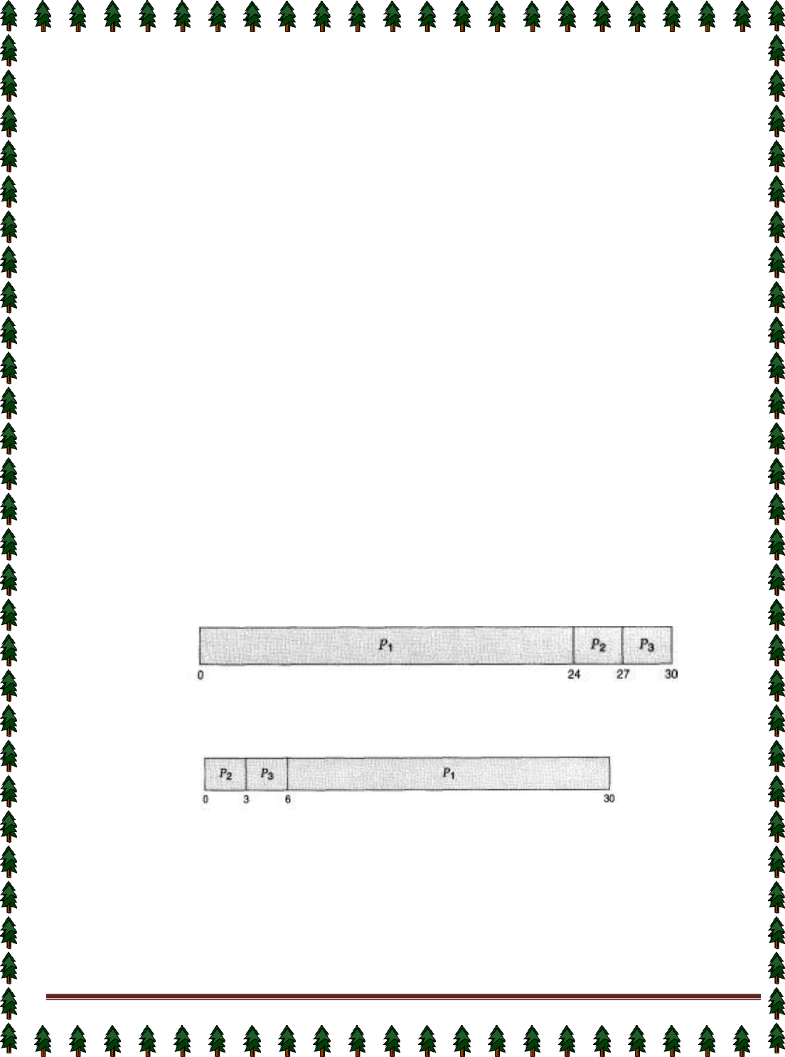
If the processes arrive in the order PI, P2, P3, and are served in FCFS order, we get the result shown in the
following Gantt chart:
The waiting time is 0 milliseconds for process PI, 24 milliseconds for process PZ, and 27 milliseconds for
process P3. Thus, the average waiting time is (0 + 24 + 27)/3 = 17 milliseconds. If the processes arrive in the
order P2, P3, Pl, however, the results will be as shown in the following Gantt chart:
The average waiting time is now (6 + 0 + 3)/3 = 3 milliseconds. This reduction is substantial. Thus, the average
waiting time under a FCFS policy is generally not minimal, and may vary substantially if the process CPU-burst
times vary greatly.
In addition, consider the performance of FCFS scheduling in a dynamic situation. Assume we have one
CPU-bound process and many I/O-bound processes. As the processes flow around the system, the following
scenario may result. The CPU-bound process will get the CPU and hold it. During this time, all the other
processes will finish their I/O and move into the ready queue, waiting for the CPU. While the processes wait in
the ready queue, the I/O devices are idle. Eventually, the CPU-bound process finishes its CPU burst and moves
to an I/O device. All the I/O-bound processes, which have very short CPU bursts, execute quickly and move
back to the I/O queues. At this point, the CPU sits idle.
Page 20
The CPU-bound process will then move back to the ready queue and be allocated the CPU. Again, all
the I/O processes end up waiting in the ready queue until the CPU-bound process is done. There is a convoy
effect, as all the other processes wait for the one big process to get off the CPU. This effect results in lower CPU
and device utilization than might be possible if the shorter processes were allowed to go first.
The FCFS scheduling algorithm is non-preemptive. Once the CPU has been allocated to a process, that
process keeps the CPU until it releases the CPU, either by terminating or by requesting I/O. The FCFS algorithm
is particularly troublesome for time-sharing systems, where each user needs to get a share of the CPU at regular
intervals. It would be disastrous to allow one process to keep the CPU for an extended period.
Shortest-Job-First Scheduling
A different approach to CPU scheduling is the shortest-job-first (SJF) scheduling algorithm. This algorithm
associates with each process the length of the latter's next CPU burst. When the CPU is available, it is assigned
to the process that has the smallest next CPU burst. If two processes have the same length next CPU burst,
FCFS scheduling is used to break the tie. Note that a more appropriate term would be the shortest next CPU
burst, because the scheduling is done by examining the length of the next CPU burst of a process, rather than its
total length. We use the term SJF because most people and textbooks refer to this type of scheduling discipline
as SJF.
As an example, consider the following set of processes, with the length of the CPU-burst time given in
milliseconds:
Process
Burst Time
PI
6
p2
8
p3
7
p4
3
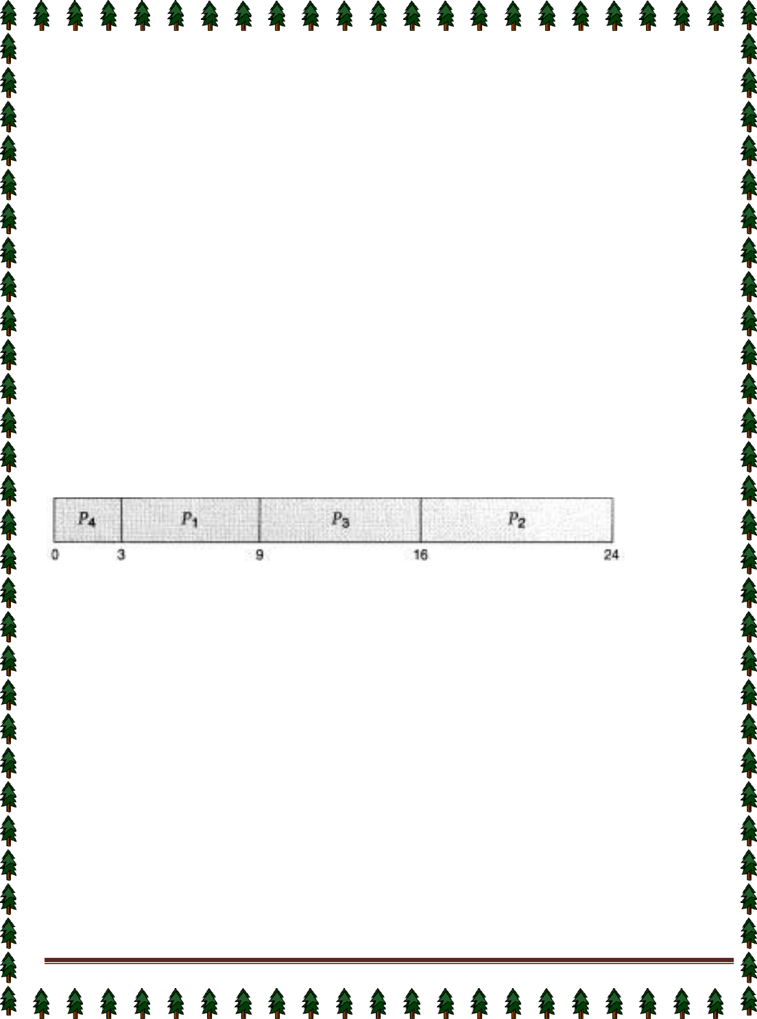
Using SJF scheduling, we would schedule these processes according to the
following Gantt chart:
The waiting time is 3 milliseconds for process PI, 16 milliseconds for process P2,9 milliseconds for process PS,
and 0 milliseconds for process Pq. Thus, the average waiting time is (3 + 16 + 9 + 0)/4 = 7 milliseconds. If we
were using the FCFS scheduling scheme, then the average waiting time would be 10.25 milliseconds.
The SJF scheduling algorithm is provably optimal, in that it gives the minimum average waiting time for a
given set of processes. By moving a short process before a long one, the waiting time of the short process
decreases more than it increases the waiting time of the long process. Consequently, the average waiting time
decreases.
The real difficulty with the SJF algorithm is knowing the length of the next CPU request. For long-term (or job)
scheduling in a batch system, we can use as the length the process time limit that a user specifies when he
submits the job.
Thus, users are motivated to estimate the process time limit accurately, since a lower value may mean
faster response. (Too low a value will cause a time-limit exceeded error and require resubmission.) SJF
scheduling is used frequently in long-term scheduling.
Although the SJF algorithm is optimal, it cannot be implemented at the level of short-term CPU scheduling.
There is no way to know the length of the next CPU burst. One approach is to try to approximate SJF
scheduling. We may not know the length of the next CPU burst, but we may be able to predict its value.We
expect that the next CPU burst will be similar in length to the previous ones.
Thus, by computing an approximation of the length of the next CPU burst, we can pick the process with
the shortest predicted CPU burst.
The SJF algorithm may be either preemptive or nonpreemptive. The choice arises when a new process
arrives at the ready queue while a previous process is executing. The new process may have a shorter next
CPU burst than what is left of the currently executing process. A preemptive SJF algorithm will preempt the
currently executing process, whereas a nonpreemptive SJF algorithm will allow the currently running process to
finish its CPU burst. Preemptive SJF scheduling is sometimes called shortest-remaining-time-first scheduling.
Page 21
As an example, consider the following four processes, with the length of the CPU-burst time given in
milliseconds:
Process Arrival Time Burst Time
P1 0 8
P2 1 4
P3 2 9
p4 3 5
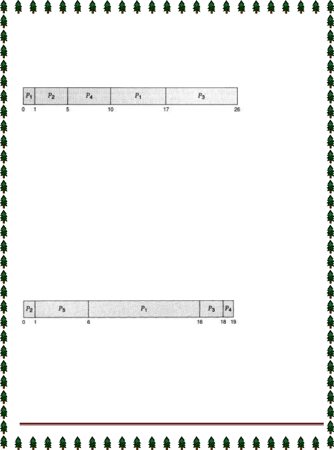
If the processes arrive at the ready queue at the times shown and need the indicated burst times, then
the resulting preemptive SJF schedule is as depicted in the following Gantt chart:
Process PI is started at time 0, since it is the only process in the queue. Process PZ arrives at time 1.
The remaining time for process P1 (7 milliseconds) is larger than the time required by process P2 (4
milliseconds), so process P1 is preempted, and process P2 is scheduled. The average waiting time for this
example is ((10 - 1) + (1 - 1) + (17 - 2) + (5 - 3))/4 = 26/4 = 6.5 milliseconds. A nonpreemptive SJF scheduling
would result in an average waiting time of 7.75 milliseconds.
Priority Scheduling
The SJF algorithm is a special case of the general priority-scheduling algorithm. A priority is associated
with each process, and the CPU is allocated to the process with the highest priority. Equal-priority processes are
scheduled in FCFS order.
An SJF algorithm is simply a priority algorithm where the priority (p) is the inverse of the (predicted) next
CPU burst. The larger the CPU burst, the lower the priority, and vice versa.
Note that we discuss scheduling in terms of high priority and low priority. Priorities are generally some
fixed range of numbers, such as 0 to 7, or 0 to 4,095. However, there is no general agreement on whether 0 is
the highest or lowest priority. Some systems use low numbers to represent low priority; others use low numbers
for high priority. This difference can lead to confusion. In this text, we use low numbers to represent high priority.
As an example, consider the following set of processes, assumed to have arrived at time 0, in the order PI, P2,
..., Ps, with the length of the CPU-burst time given in milliseconds:
Process
Burst
Time Priority
P1
10
3
p2
1
1
p3
2
4
P4
1
5
P5
5
2
Using priority scheduling, we would schedule these processes according to the following Gantt chart:
The average waiting time is 8.2 milliseconds. Priorities can be defined either internally or externally.
Internally defined priorities use some measurable quantity or quantities to compute the priority of a process.
For example, time limits, memory requirements, the number of open files, and the ratio of average I/O
burst to average CPU burst have been used in computing priorities. External priorities are set by criteria that are
external to the operating system, such as the importance of the process, the type and amount of funds being
paid for computer use, the department sponsoring the work, and other, often political, factors.
Priority scheduling can be either preemptive or nonpreemptive. When a process arrives at the ready
queue, its priority is compared with the priority of the currently running process. A preemptive priority-scheduling
algorithm will preempt the CPU if the priority of the newly arrived process is higher than the priority of the
currently running process. A nonpreemptive priority-scheduling
algorithm will simply put the new process at the head of the ready queue.
A major problem with priority-scheduling algorithms is indefinite blocking (or starvation). A process that is
ready to run but lacking the CPU can be considered blocked-waiting for the CPU. A priority-scheduling algorithm
can leave some low-priority processes waiting indefinitely for the CPU.
Page 22
A solution to the problem of indefinite blockage of low-priority processes is aging. Aging is a technique of
gradually increasing the priority of processes that wait in the system for a long time. For example, if priorities
range from 127 (low) to 0 (high), we could decrement the priority of a waiting process by 1 every 15 minutes.
Eventually, even a process with an initial priority of 127 would have the highest priority in the system and would
be executed. In fact, it would take no more than 32 hours for a priority 127 process to age to a priority 0 process.
Round-Robin Scheduling
The round-robin (RR) scheduling algorithm is designed especially for timesharing systems. It is similar to
FCFS scheduling, but preemption is added to switch between processes. A small unit of time, called a time
quantum (or time slice), is defined. A time quantum is generally from 10 to 100 milliseconds. The ready queue is
treated as a circular queue. The CPU scheduler goes around the ready queue, allocating the CPU to each
process for a time interval of up to 1 time quantum.
To implement RR scheduling, we keep the ready queue as a FIFO queue of processes. New processes
are added to the tail of the ready queue. The CPU scheduler picks the first process from the ready queue, sets a
timer to interrupt after 1 time quantum, and dispatches the process.
One of two things will then happen. The process may have a CPU burst of less than 1 time quantum. In
this case, the process itself will release the CPU voluntarily. The scheduler will then proceed to the next process
in the ready queue. Otherwise, if the CPU burst of the currently running process is longer than 1 time quantum,
the timer will go off and will cause an interrupt to the operating system. A context switch will be executed, and
the process will be put at the tail of the ready queue. The CPU scheduler will then select the next process in the
ready queue.
The average waiting time under the RR policy, however, is often quite long.
Consider the following set of processes that arrive at time 0, with the length of the CPU-burst time given
in milliseconds:
Process Burst Time
PI 24
P2 3
P3 3
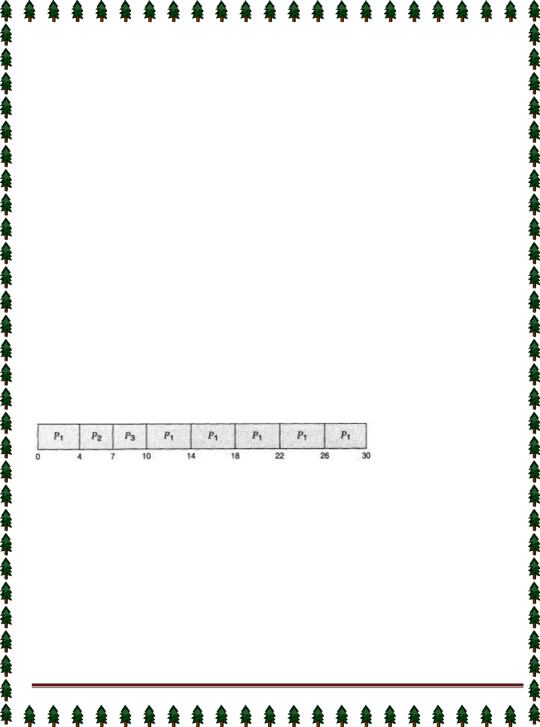
If we use a time quantum of 4 milliseconds, then process P1 gets the first 4 milliseconds. Since it requires
another 20 milliseconds, it is preempted after the first time quantum, and the CPU is given to the next process in
the queue, process P2. Since process P2 does not need 4 milliseconds, it quits before its time quantum expires.
The CPU is then given to the next process, process P3. Once each process has received 1 time quantum, the
CPU is returned to process P1 for an additional time quantum. The resulting RR schedule is
The average waiting time is 17/3 = 5.66 milliseconds.
In the RR scheduling algorithm, no process is allocated the CPU for more than 1 time quantum in a row.
If a process' CPU burst exceeds 1 time quantum, that process is preempted and is put back in the ready queue.
The RR scheduling algorithm is preemptive.
If there are n processes in the ready queue and the time quantum is q, then each process gets l/n of the
CPU time in chunks of at most q time units. Each process must wait no longer than (n - 1) x q time units until its
next time quantum. For example, if there are five processes, with a time quantum of 20 milliseconds, then each
process will get up to 20 milliseconds every 100
milliseconds.
The performance of the RR algorithm depends heavily on the size of the time quantum. At one extreme,
if the time quantum is very large (infinite), the RR policy is the same as the FCFS policy. If the time quantum is
very small (say 1 microsecond), the RR approach is called processor sharing, and appears (in theory) to the
users as though each of n processes has its own processor running at l/n the speed of the real processor. This
approach was used in Control Data Corporation (CDC) hardware to implement 10 peripheral processors with
only one set of hardware and 10 sets of registers. The hardware executes one instruction for one set of registers,
then goes on to the next. This cycle continues, resulting in 10 slow processors rather than one fast processor.
Multilevel Queue Scheduling
Another class of scheduling algorithms has been created for situations in which processes are easily
classified into different groups. For example, a common division is made between foreground (or interactive)

Page 23
processes and background (or batch) processes. These two types of processes have different response-time
requirements, and so might have different scheduling needs. In addition, foreground processes may have priority
(or externally defined) over background processes.
Preemptive Vs Nonpreemptive Scheduling
The Scheduling algorithms can be divided into two categories with respect to how they deal with clock
interrupts.
Nonpreemptive Scheduling: A scheduling discipline is nonpreemptive , if once a process has been used the
CPU, the CPU cannot be taken away from that process.
Preemptive Scheduling: A scheduling discipline is preemptive, if once a process has been used the CPU, the
CPU can taken away.
Page 24
Lecture #13,#14
Thread
A thread, sometimes called a lightweight process (LWP), is a basic unit of CPU utilization; it comprises a
thread ID, a program counter, a register set, and a stack. It shares with other threads belonging to the same
process its code section, data section, and other operating-system resources, such as open files and signals. A
traditional (or heavyweight) process has a single thread of control. If the process has multiple threads of control,
it can do more than one task at a time.
Motivation
Many software packages that run on modern desktop PCs are multithreaded.An application typically is
implemented as a separate process with several thread of control.
Single-threaded and multithreaded
Ex: A web browser might have one thread display images or text while another thread retrieves data
from the network. A word processor may have a thread for displaying graphics, another thread for reading
keystrokes from the user, and a third thread for performing spelling and grammar checking in the background.
In certain situations a single application may be required to perform several similar tasks. For example, a
web server accepts client requests for web pages, images, sound, and so forth. A busy web server may have
several (perhaps hundreds) of clients concurrently accessing it. If the web server ran as a traditional single-
threaded process, it would be able to service only one client at a time.
One solution is to have the server run as a single process that accepts requests. When the server
receives a request, it creates a separate process to service that request. In fact, this process-creation method
was in common use before threads became popular. Process creation is very heavyweight, as was shown in the
previous chapter. If the new process will perform the same tasks as the existing process, why incur all that
overhead? It is generally more efficient for one process that contains multiple threads to serve the same
purpose. This approach would multithread the web-server process. The server would create a separate thread
that would listen for client requests; when a request was made, rather than creating another process, it would
create another thread to service the request.
Threads also play a vital role in remote procedure call (RPC) systems. RPCs allow inter-process
communication by providing a communication mechanism similar to ordinary function or procedure calls.
Typically, RPC servers are multithreaded. When a server receives a message, it services the message using a
separate thread. This allows the server to service several concurrent requests.
Benefits
The benefits of multithreaded programming can be broken down into four major categories:
1.
Responsiveness: Multithreading an interactive application may allow a program to continue running even if
part of it is blocked or is performing a lengthy operation, thereby increasing responsiveness to the user. For
instance, a multithreaded web browser could still allow user interaction
in one thread while an image is being loaded in another thread.

Page 25
2.
Resource sharing: By default, threads share the memory and the resources of the process to which they
belong. The benefit of code sharing is that it allows an application to have several different threads of activity all
within the same address space.
3.
Economy: Allocating memory and resources for process creation is costly. Alternatively, because threads
share resources of the process to which they belong, it is more economical to create and context switch threads.
It can be difficult to gauge empirically the difference in overhead for creating and maintaining a process rather
than a thread, but in general it is much more time consuming to create and manage processes than threads. In
Solaris 2, creating a process is about 30 times slower than is creating a thread, and context switching is about
five times slower.
4.
Utilization of multiprocessor architectures: The benefits of multithreading can be greatly increased in a
multiprocessor architecture, where each thread may be running in parallel on a different processor. A single-
threaded process can only run on one CPU, no matter how many are available.
Multithreading on a multi-CPU machine increases concurrency. In a single processor architecture, the
CPU generally moves between each thread so quickly as to create an illusion of parallelism, but in reality only
one thread is running at a time.
The OS supports the threads that can provided in following two levels:
User-Level Threads
User-level threads implement in user-level libraries, rather than via systems calls, so thread switching
does not need to call operating system and to cause interrupt to the kernel. In fact, the kernel knows nothing
about user-level threads and manages them as if they were single-threaded processes.
Advantages:
User-level threads do not require modification to operating systems.
Simple Representation: Each thread is represented simply by a PC, registers, stack and a small control
block, all stored in the user process address space.
Simple Management: This simply means that creating a thread, switching between threads and
synchronization between threads can all be done without intervention of the kernel.
Fast and Efficient: Thread switching is not much more expensive than a procedure call.
Disadvantages:
There is a lack of coordination between threads and operating system kernel.
User-level threads require non-blocking systems call i.e., a multithreaded kernel.
Kernel-Level Threads
In this method, the kernel knows about and manages the threads. Instead of thread table in each process, the
kernel has a thread table that keeps track of all threads in the system. Operating Systems kernel provides
system call to create and manage threads.
Advantages:
Because kernel has full knowledge of all threads, Scheduler may decide to give more time to a process
having large number of threads than process having small number of threads.
Kernel-level threads are especially good for applications that frequently block.
Disadvantages:
The kernel-level threads are slow and inefficient. For instance, threads operations are hundreds of times
slower than that of user-level threads.
Since kernel must manage and schedule threads as well as processes. It require a full thread control block
(TCB) for each thread to maintain information about threads. As a result there is significant overhead and
increased in kernel complexity.
Multithreading Models
Many systems provide support for both user and kernel threads, resulting in different multithreading
models. We look at three common types of threading implementation.
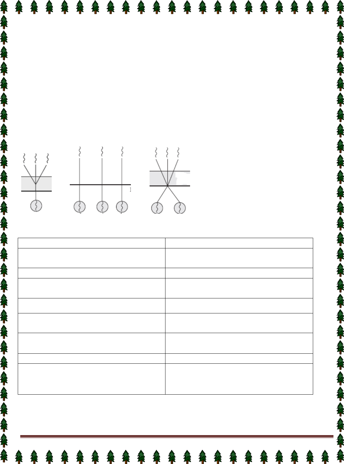
Many-to-One Model
The many-to-one model maps many user-level threads to one kernel thread. Thread management is
done in user space, so it is efficient, but the entire process will block if a thread makes a blocking system call.
Also, because only one thread can access the kernel at a time, multiple threads are unable to run in parallel on
multiprocessors.
One-to-one Model
Page 26
The one-to-one model maps each user thread to a kernel thread. It provides more concurrency than the
many-to-one model by allowing another thread to run when a thread makes a blocking system call; it also allows
multiple threads to run in parallel on multiprocessors. The only drawback to this model is that creating a user
thread requires creating the corresponding kernel thread. Because the overhead of creating kernel threads can
burden the performance of an application, most implementations of this model restrict the number of threads
supported by the system. Windows NT, Windows 2000, and OS/2 implement the one-to-one model.
Many-to-Many Model
The many-to-many model multiplexes many user-level threads to a smaller or equal number of kernel
threads. The number of kernel threads may be specific to either a particular application or a particular machine
(an application may be allocated more kernel threads on a multiprocessor than on a uniprocessor). Whereas the
many-to-one model allows the developer to create as many user threads as she wishes, true concurrency is not
gained because the kernel can schedule only one thread at a time. The one-to-one model allows for greater
concurrency, but the developer has to be careful not to create too many threads within an application (and in
some instances may be limited in the number of threads she can create). The many-to-many model suffers from
neither of these shortcomings: Developers can create as many user threads as necessary, and the
corresponding kernel threads can run in parallel on a multiprocessor.
(Diagram of
many-to-one model, one-to-one model and many-to-many model
)
Process vs. Thread
Process
Thread
1.Process cannot share the same memory
area(address space)
1.Threads can share memory and files.
2.It takes more time to create a process
2.It takes less time to create a thread.
3.It takes more time to complete the execution and
terminate.
3.Less time to terminate.
4.Execution is very slow.
4.Execution is very fast.
5.It takes more time to switch between two
processes.
5.It takes less time to switch between two threads.
6.System calls are required to communicate each
other
6.System calls are not required.
7.It requires more resources to execute.
7.Requires fewer resources.
8.Implementing the communication between
processes is bit more difficult.
8.Communication between two threads are very
easy to implement because threads share the
memory

Page 29
Lecture #15
Inter-process Communication (IPC)
Mechanism for processes to communicate and to synchronize their actions.
Message system – processes communicate with each other without resorting to shared variables.
IPC facility provides two operations:
1.
send(message) – message size fixed or variable
2.
receive(message)
If P and Q wish to communicate, they need to:
1.
establish a communication link between them
2.
exchange messages via send/receive
Implementation of communication link
1.
physical (e.g., shared memory, hardware bus)
2.
logical (e.g., logical properties)
Direct Communication
Processes must name each other explicitly:
✦ send (P, message) – send a message to process P
✦ receive(Q, message) – receive a message from process Q Properties of communication link
✦ Links are established automatically.
✦ A link is associated with exactly one pair of communicating processes.
✦ Between each pair there exists exactly one link.
✦ The link may be unidirectional, but is usually bi-directional.
Indirect Communication
Messages are directed and received from mailboxes (also referred to as ports).
✦ Each mailbox has a unique id.
✦ Processes can communicate only if they share a mailbox.
Properties of communication link
✦ Link established only if processes share a common mailbox
✦ A link may be associated with many processes.
✦ Each pair of processes may share several communication links.
✦ Link may be unidirectional or bi-directional.
Operations
✦ create a new mailbox
✦ send and receive messages through mailbox
✦ destroy a mailbox
Primitives are defined as:
send(A, message) – send a message to mailbox A
receive(A, message) – receive a message from mailbox A
Mailbox sharing
✦ P1, P2, and P3 share mailbox A.
✦ P1, sends; P2 and P3 receive.
✦ Who gets the message?
Solutions
✦ Allow a link to be associated with at most two processes.
✦ Allow only one process at a time to execute a receive operation.
✦ Allow the system to select arbitrarily the receiver. Sender is notified who the receiver was.
Concurrent Processes
The concurrent processes executing in the operating system may be either independent processes or
cooperating processes. A process is independent if it cannot affect or be affected by the other processes
executing in the system.Clearly, any process that does not share any data (temporary or persistent) with any
other process is independent. On the other hand, a process is cooperating if it can affect or be affected by the

Page 30

Page 31
other processes executing in the system.Clearly, any process that shares data with other processes is a
cooperating process.
We may want to provide an environment that allows process cooperation
for several reasons:
Information sharing: Since several users may be interested in the same piece of information (for instance, a
shared file), we must provide an environment to allow concurrent access to these types of resources.
Computation speedup: If we want a particular task to run faster, we must break it into subtasks, each of wluch
will be executing in parallel with the others. Such a speedup can be achieved only if the computer has multiple
processing elements (such as CPUS or I/O channels).
Modularity: We may want to construct the system in a modular fashion,dividing the system functions into
separate processes or threads.
Convenience: Even an individual user may have many tasks on which to work at one time. For instance, a user
may be editing, printing, and compiling in parallel.

Page 32
Lecture # 16
Message-Passing System
The function of a message system is to allow processes to communicate with one another without the
need to resort to shared data. We have already seen message passing used as a method of communication in
microkernels. In this scheme, services are provided as ordinary user processes. That is, the services operate
outside of the kernel. Communication among the user processes is accomplished through the passing of
messages. An IPC facility provides at least the two operations: send (message) and receive (message).
Messages sent by a process can be of either fixed or variable size. If only fixed-sized messages can be
sent, the system-level implementation is straightforward. This restriction, however, makes the task of
programming more difficult. On the other hand, variable-sized messages require a more complex system-level
implementation, but the programming task becomes simpler.
If processes P and Q want to communicate, they must send messages to and receive messages from
each other; a communication link must exist between them. This link can be implemented in a variety of ways.
We are concerned here not with the link's physical implementation, but rather with its logical implementation.
Here are several methods for logically implementing a link and the send/receive operations:
Direct or indirect communication
Symmetric or asymmetric communication
Automatic or explicit buffering
Send by copy or send by reference
Fixed-sized or variable-sized messages
We look at each of these types of message systems next.
Synchronization
Communication between processes takes place by calls to send and receive primitives. There are different
design options for implementing each primitive. Message passing may be either blocking or nonblocking-also
known as synchronous and asynchronous.
Blocking send: The sending process is blocked until the message is received by the receiving process or by the
mailbox.
Nonblocking send: The sending process sends the message and resumes operation.
Blocking receive: The receiver blocks until a message is available.
Nonblocking receive: The receiver retrieves either a valid message or a null.
Different combinations of send and receive are possible. When both the send and receive are blocking,
we have a rendezvous between the sender and the receiver.
Buffering
Whether the communication is direct or indirect, messages exchanged by communicating processes reside in a
temporary queue. Basically, such a queue can be implemented in three ways:
Zero capacity: The queue has maximum length 0; thus, the link cannot have any messages waiting in it. In this
case, the sender must block until the recipient receives the message.
Bounded capacity: The queue has finite length n; thus, at most n messages can reside in it. If the queue is not
full when a new message is sent, the latter is placed in the queue (either the message is copied or a pointer to
the message is kept), and the sender can continue execution without waiting. The link has a finite capacity,
however. If the link is full, the sender must block until space is available in the queue.
Unbounded capacity: The queue has potentially infinite length; thus, any number of messages can wait in it.
The sender never blocks.The zero-capacity case is sometimes referred to as a message system with no
buffering; the other cases are referred to as automatic buffering.
Client-Server Communication
Sockets
Remote Procedure Calls
Remote Method Invocation (Java)

Page 33
Lecture # 17
Process Synchronization
A situation where several processes access and manipulate the same data concurrently and the
outcome of the execution depends on the particular order in which the access takes place, is called a race
condition.
Producer-Consumer Problem
Paradigm for cooperating processes, producer process produces information that is consumed by a
consumer process.
To allow producer and consumer processes to run concurrently, we must have available a buffer of
items that can be filled by the producer and emptied by the consumer. A producer can produce one item while
the consumer is consuming another item. The producer and consumer must be synchronized, so that the
consumer does not try to consume an item that has not yet been produced. In this situation, the consumer must
wait until an item is produced.
✦ unbounded-buffer places no practical limit on the size of the buffer.
✦ bounded-buffer assumes that there is a fixed buffer size.
Bounded-Buffer – Shared-Memory Solution
The consumer and producer processes share the following variables.
Shared data
#define BUFFER_SIZE 10
Typedef struct
{
. . .
} item;
item buffer[BUFFER_SIZE];
int in = 0;
int out = 0;
Solution is correct, but can only use BUFFER_SIZE-1 elements.
The shared buffer is implemented as a circular array with two logical pointers: in and out. The variable in points
to the next free position in the buffer; out points to the first full position in the buffer. The buffer is empty when in
== out ; the buffer is full when ((in + 1) % BUFFERSIZE) == out.
The code for the producer and consumer processes follows. The producer process has a local variable
nextproduced in which the new item to be produced is stored:
Bounded-Buffer – Producer Process
item nextProduced;
while (1)
{
while (((in + 1) % BUFFER_SIZE) == out)
; /* do nothing */
buffer[in] = nextProduced;
in = (in + 1) % BUFFER_SIZE;
}
Bounded-Buffer – Consumer Process
item nextConsumed;

Page 34
while (1)
{
while (in == out)
; /* do nothing */
nextConsumed = buffer[out];
out = (out + 1) % BUFFER_SIZE;
}
The critical section problem
Consider a system consisting of n processes {Po,P1, ..., Pn-1). Each process has a segment of code,
called a critical section, in which the process may be changing common variables, updating a table, writing a
file, and so on. The important feature of the system is that, when one process is executing in its critical section,
no other process is to be allowed to execute in its critical section. Thus, the execution of critical sections by the
processes is mutually exclusive in time. The critical-section problem is to design a protocol that the processes
can use to cooperate. Each process must request permission to enter its critical section. The section of code
implementing this request is the entry section. The critical section may be followed by an exit section. The
remaining code is the remainder section.
do{
Entry section
Critical section
Exit section
Remainder section
}while(1);
A solution to the critical-section problem must satisfy the following three requirements:
1.
Mutual Exclusion: If process Pi is executing in its critical section, then no other processes can be executing
in their critical sections.
2.
Progress: If no process is executing in its critical section and some processes wish to enter their critical
sections, then only those processes that are not executing in their remainder section can participate in the
decision on which will enter its critical section next, and this selection cannot be postponed indefinitely.
3.
Bounded Waiting: There exists a bound on the number of times that other processes are allowed to enter
their critical sections after a process has made a request to enter its critical section and before that request is
granted.

Page 35
Lecture # 18
Peterson’s solution
Peterson’s solution is a software based solution to the critical section problem.
Consider two processes P0 and P1. For convenience, when presenting Pi, we use Pi to denote the other
process; that is, j == 1 - i.
The processes share two variables:
boolean flag [2] ;
int turn;
Initially flag [0] = flag [1] = false, and the value of turn is immaterial (but is either 0 or 1). The structure of process
Pi is shown below.
do{
flag[i]=true
turn=j
while(flag[j] && turn==j);
critical section
flag[i]=false
Remainder section
}while(1);
To enter the critical section, process Pi first sets flag [il to be true and then sets turn to the value j,
thereby asserting that if the other process wishes to enter the critical section it can do so. If both processes try to
enter at the same time, turn will be set to both i and j at roughly the same time. Only one of these assignments
will last; the other will occur, but will be overwritten immediately. The eventual value of turn decides which of the
two processes is allowed to enter its critical section first.
We now prove that this solution is correct. We need to show that:
1.
Mutual exclusion is preserved,
2.
The progress requirement is satisfied,
3.
The bounded-waiting requirement is met.
To prove property 1, we note that each Pi enters its critical section only if either flag [jl == false or turn ==
i.
Also note that, if both processes can be executing in their critical sections at the same time, then flag [i] ==flag
[jl == true. These two observations imply that P0 and P1 could not have successfully executed their while
statements at about the same time, since the value of turn can be either 0 or 1, but cannot be both. Hence, one
of the processes say Pj-must have successfully executed the while statement, whereas Pi had to execute at
least one additional statement ("turn == j"). However, since, at that time, flag [j] == true, and turn == j, and this
condition will persist as long as Pi is in its critical section, the result follows:
To prove properties 2 and 3, we note that a process Pi can be prevented from entering the critical
section only if it is stuck in the while loop with the condition flag [j] == true and turn == j; this loop is the only one.
If Pi is not ready to enter the critical section, then flag [ j ] == false and Pi can enter its critical section. If Pi has
set flag[j] to true and is also executing in its while statement, then either turn == i or turn == j. If turn == i, then Pi
will enter the critical section. If turn == j, then Pi will enter the critical section. However, once Pi exits its critical
section, it will reset flag [ jl to false, allowing Pi to enter its critical section. If Pi resets flag [ j 1 to true, it must also
set turn to i.
Thus, since Pi does not change the value of the variable turn while executing the while statement, Pi will
enter the critical section (progress) after at most one entry by Pi (bounded waiting).

Page 36
Lecture # 19
Synchronization Hardware
As with other aspects of software, hardware features can make the programming task easier and
improve system efficiency. In this section, we present some simple hardware instructions that are available on
many systems, and show how they can be used effectively in solving the critical-section problem.
The definition of the TestAndSet instruction.
boolean TestAndSet(boo1ean &target)
{
boolean rv = target;
target = true;
return rv;
}
The critical-section problem could be solved simply in a uniprocessor environment if we could forbid
interrupts to occur while a shared variable is being modified. In this manner, we could be sure that the current
sequence of instructions would be allowed to execute in order without preemption. No other instructions would
be run, so no unexpected modifications could be made to the shared variable.
Unfortunately, this solution is not feasible in a multiprocessor environment. Disabling interrupts on a
multiprocessor can be time-consuming, as the message is passed to all the processors. This message passing
delays entry into each critical section, and system efficiency decreases. Also, consider the effect on a system's
clock, if the clock is kept updated by interrupts.
Many machines therefore provide special hardware instructions that allow us either to test and modify
the content of a word, or to swap the contents of two words, atomically-that is, as one uninterruptible unit. We
can use these special instructions to solve the critical-section problem in a relatively simple manner. Rather than
discussing one specific instruction for one specific machine, let us abstract the main concepts behind these
types of instructions.
The TestAndSet instruction can be defined as shown in code. The important characteristic is that this instruction
is executed atomically. Thus, if two TestAndSet instructions are executed simultaneously (each on a different
CPU), they will be executed sequentially in some arbitrary order.
Mutual-exclusion implementation with TestAndSet
do{
while(TestAndSet(lock));
critical section
lock=false
Remainder section
}while(1);
void Swap(boo1ean &a, boolean &b) {
boolean temp = a;
a = b;
b = temp}
If the machine supports the TestAndSet instruction, then we can implement mutual exclusion by
declaring a Boolean variable lock, initialized to false.
If the machine supports the Swap instruction, then mutual exclusion can be provided as follows. A global
Boolean variable lock is declared and is initialized to false. In addition, each process also has a local Boolean
variable key.

Page 37
Lecture # 20
Semaphores
The solutions to the critical-section problem presented before are not easy to generalize to more
complex problems. To overcome this difficulty, we can use a synchronization tool called a semaphore. A
semaphore S is an integer variable that, apart from initialization, is accessed only through two standard atomic
operations: wait and signal. These operations were originally termed P (for wait; from the Dutch proberen, to
test) and V (for signal; from verhogen, to increment). The classical definition of wait in pseudocode is
wait(S) {
while (S <= 0)
; // no-op
S --;
}
The classical definitions of signal in pseudocode is
Signal(S){
S++;
}
Modifications to the integer value of the semaphore in the wait and signal operations must be executed
indivisibly. That is, when one process modifies the semaphore value, no other process can simultaneously
modify that same semaphore value. In addition, in the case of the wait (S), the testing of the integer value of S (S
5 O), and its possible modification (S--), must also be executed without interruption.
Usage
We can use semaphores to deal with the n-process critical-section problem. The n processes share a
semaphore, mutex (standing for mutual exclusion), initialized to 1. Each process Pi is organized as shown in
Figure.We can also use semaphores to solve various synchronization problems.
For example, consider two concurrently running processes: PI with a statement S1 and P2 with a statement S2.
Suppose that we require that S2 be executed only after S1 has completed. We can implement this scheme
readily by letting P1 and P2 share a common semaphore synch, initialized to 0, and by inserting the statements
in process PI, and the statements
wait (synch) ;
s2;
in process P2. Because synch is initialized to 0, P2 will execute S2 only after PI
has invoked signal (synch) , which is after S1.
s1;
signal (synch) ;
do {
wait (mutex) ;
critical section
signal (mutex) ;
remainder section
} while (1);
Mutual-exclusion implementation with semaphores.
Implementation
The main disadvantage of the mutual-exclusion solutions and of the semaphore definition given here, is
that they all require busy waiting. While a process is in its critical section, any other process that tries to enter its

Page 38
critical section must loop continuously in the entry code. This continual looping is clearly a problem in a real
multiprogramming system, where a single CPU is
shared among many processes. Busy waiting wastes CPU cycles that some other process might be able to use
productively. This type of semaphore is also called a spinlock (because the process "spins" while waiting for the
lock). Spinlocks are useful in multiprocessor systems. The advantage of a spinlock is that no context switch is
required when a process must wait on a lock, and a context switch may take considerable time. Thus, when
locks are expected to be held for short times, spinlocks are useful.
To overcome the need for busy waiting, we can modify the definition of the wait and signal semaphore
operations. When a process executes the wait operation and finds that the semaphore value is not positive, it
must wait. However, rather than busy waiting, the process can block itself. The block operation places a process
into a waiting queue associated with the semaphore, and the state of the process is switched to the waiting state.
Then, control is transferred to the CPU scheduler, which selects another process to execute.
A process that is blocked, waiting on a semaphore S, should be restarted when some other process
executes a signal operation. The process is restarted by a wakeup operation, which changes the process from
the waiting state to the ready state. The process is then placed in the ready queue. (The CPU may or may not be
switched from the running process to the newly ready process, depending on the CPU-scheduling algorithm.)
To implement semaphores under this definition, we define a semaphore as a "C" struct:
typedef struct {
int value ;
struct process *L;
) semaphore;
Each semaphore has an integer value and a list of processes. When a process must wait on a semaphore, it is
added to the list of processes. A signal operation removes one process from the list of waiting processes and
awakens that process.
The wait semaphore operation can now be defined as
void wait(semaphore S) {
S.value--;
if (S.value < 0) {
add this process to S . L;
block() ;
}
The signal semaphore operation can now be defined as
void signal(semaphore S) {
S.value++;
if (S.value <= 0) {
remove a process P from S . L ;
wakeup (PI) ;
}
The block operation suspends the process that invokes it. The wakeup(P1) operation resumes the execution of a
blocked process P. These two operations are provided by the operating system as basic system calls.
Binary Semaphores
The semaphore construct described in the previous sections is commonly known as a counting semaphore,
since its integer value can range over an unrestricted domain. A binary semaphore is a semaphore with an
integer value that can range only between 0 and 1. A binary semaphore can be simpler to implement than a
counting semaphore, depending on the underlying hardware architecture. We will now show how a counting
semaphore can be implemented using binary semaphores. Let S be a counting semaphore.
To implement it in terms of binary semaphores we need the following data structures:
binary-semaphore S1, S2;

Page 39
int C;
Initially S1 = 1, S2 = 0, and the value of integer C is set to the initial value of the counting semaphore S.
The wait operation on the counting semaphore S can be implemented as follows:
wait (S1) ;
C--;
i f (C < 0) {
signal(S1) ;
wait (S2) ;
}
signal(S1);
The signal operation on the counting semaphore S can be implemented as follows:
w a i t (S1) ;
C++ ;
i f (C <= 0)
signal (S2) ;
e l s e
signal (S1) ;
Classic Problems of Synchronization
We present a number of different synchronization problems as examples for a large class of concurrency-control
problems. These problems are used for testing nearly every newly proposed synchronization
scheme.Semaphores are used for synchronization in our solutions.
The Bounded-Buffer Problem
The bounded-buffer problem is commonly used to illustrate the power of synchronization primitives. We
present here a general structure of this scheme, without committing ourselves to any particular implementation.
We assume that the pool consists of n buffers, each capable of holding one item. The mutex semaphore
provides mutual exclusion for accesses to the buffer pool and is initialized to the value 1. The empty and full
semaphores count the number of empty and full buffers, respectively. The semaphore empty is initialized to the
value n; the semaphore f u l l is initialized to the value 0.
The code for the producer process is
do{
produce an item in nextp
...
wait (empty) ;
wait (mutex) ;
...
add nextp to buffer
. . .
signal(mutex);
signal (full) ;
) while (1);
The code for the consumer process is
do{
wait (full) ;
wait (mutex) ;
. . .

Page 40
remove an item from buffer to nextc
...
signal (mutex) ;
signal (empty) ;
...
consume the item in nextc
...
) while (1);
Note the symmetry between the producer and the consumer. We can interpret this code as the producer
producing full buffers for the consumer, or as the consumer producing empty buffers for the producer.
Lecture # 22
The Readers- Writers Problem
A data object (such as a file or record) is to be shared among several concurrent processes. Some of
these processes may want only to read the content of the shared object, whereas others may want to update
(that is, to read and write) the shared object. We distinguish between these two types of processes by referring
to those processes that are interested in only reading as readers, and to the rest as writers. Obviously, if two
readers access the shared data object simultaneously, no adverse effects will result. However, if a writer and
some other process (either a reader or a writer) access the shared object simultaneously, chaos may ensue.
To ensure that these difficulties do not arise, we require that the writers have exclusive access to the
shared object. This synchronization problem is referred to as the readers-writers problem. Since it was originally
stated, it has been used to test nearly every new synchronization primitive. The readers-writers problem has
several variations, all involving priorities. The simplest one, referred to as the first readers-writers problem,
requires that no reader will be kept waiting unless a writer has already obtained permission to use the shared
object. In other words, no reader should wait for other readers to finish simply because a writer is waiting. The
second readers-writers problem requires that, once a writer is ready, that writer performs its write as soon as
possible. In other words, if a writer is waiting to access the object, no new readers may start reading.
A solution to either problem may result in starvation. In the first case, writers may starve; in the second
case, readers may starve. For this reason, other variants of the problem have been proposed. In this section, we
present a solution to the first readers-writers problem.
In the solution to the first readers-writers problem, the reader processes
share the following data structures:
semaphore mutex, wrt;
int readcount;
The semaphores mutex and w r t are initialized to 1; readcount is initialized to 0. The semaphore w r t is
common to both the reader and writer processes. The mutex semaphore is used to ensure mutual exclusion
when the variable readcount is updated. The readcount variable keeps track of how many processes are
currently reading the object. The semaphore wrt functions as a mutual-exclusion semaphore for the writers. It is
also used by the first or last reader that enters or exits the critical section. It is not used by readers who enter or
exit while other readers are in their critical sections.
The code for a writer process is
do{
wait (wrt) ;
. . .
writing is performed
...
signal(wrt);
}while(1);
The code for a reader process is

Page 41
do{
wait (mutex) ;
readcount++;
if (readcount == 1)
wait (wrt) ;
signal (mutex) ;
. . .
reading is performed
...
wait (mutex) ;
readcount--;
if (readcount == 0)
signal(wrt1;
signal (mutex) ;
}while(1);
Note that, if a writer is in the critical section and n readers are waiting, then one reader is queued on wrt, and n -
1 readers are queued on mutex. Also observe that, when a writer executes signal (wrt), we may resume the
execution of either the waiting readers or a single waiting writer.
Lecture #23
The Dining-Philosophers Problem
Consider five philosophers who spend their lives thinking and eating. The philosophers share a common
circular table surrounded by five chairs, each belonging to one philosopher. In the center of the table is a bowl of
rice, and the table is laid with five single chopsticks. When a philosopher thinks, she does not interact with her
colleagues. From time to time, a philosopher gets hungry and tries to pick up the two chopsticks that are closest
to her (the chopsticks that are between her and her left and right neighbors). A philosopher may pick up only one
chopstick at a time. Obviously, she cannot pick up a chopstick that is already in the hand of a neighbor. When a
hungry philosopher has both her chopsticks at the same time, she eats without releasing her chopsticks. When
she is finished eating, she puts down both of her chopsticks and starts thinking again.
The structure of philosopher i
do {
wait (chopstick[i]) ;
wait (chopstick[(i+1) % 5] ) ;
...
eat
. . .
signal (chopstick [i] ;
signal(chopstick[(i+1) % 5] ) ;
. . .
think
...
) while (1);
.
The dining-philosophers problem is considered a classic synchronization problem, neither because of its
practical importance nor because computer scientists dislike philosophers, but because it is an example of a
large class of concurrency-control problems. It is a simple representation of the need to allocate several
resources among several processes in a deadlock- and starvation free manner.
One simple solution is to represent each chopstick by a semaphore. A philosopher tries to grab the chopstick by
executing a wait operation on that semaphore; she releases her chopsticks by executing the signal operation on
the appropriate semaphores. Thus, the shared data are

Page 42
semaphore chopstick [5] ; where all the elements of chopstick are initialized to 1.
Although this solution guarantees that no two neighbors are eating simultaneously,
it nevertheless must be rejected because it has the possibility of creating a deadlock. Suppose that all five
philosophers become hungry simultaneously, and each grabs her left chopstick. All the elements of chopstick will
now be equal to 0. When each philosopher tries to grab her right chopstick, she will be delayed forever.
Use an asymmetric solution; that is, an odd philosopher picks up first her left chopstick and then her right
chopstick, whereas an even philosopher picks up her right chopstick and then her left chopstick.Finally, any
satisfactory solution to the dining-philosophers problem must guard against the possibility that one of the
philosophers will starve to death.
Lecture #24
Monitors
Another high-level synchronization construct is the monitor type. A monitor is characterized by a set of
programmer-defined operators. The representation of a monitor type consists of declarations of variables whose
values define the state of an instance of the type, as well as the bodies of procedures or functions that
implement operations on the type. The syntax of a monitor is
.
The representation of a monitor type cannot be used directly by the various processes. Thus, a procedure
defined within a monitor can access only those variables declared locally within the monitor and its formal
parameters. Similarly, the local variables of a monitor can be accessed by only the local procedures.
The monitor construct ensures that only one process at a time can be active within the monitor. Consequently,
the programmer does not need to code this synchronization constraint explicitly. However, the monitor construct,
as defined so far, is not sufficiently powerful for modeling some
synchronization schemes. For this purpose, we need to define additional synchronization mechanisms. These
mechanisms are provided by the condition operations construct. A programmer who needs to write her own
tailor-made synchronization scheme can define one or more variables of type condition:
condition x, y;
The only operations that can be invoked on a condition variable are wait and signal. The operation means that
the process invoking this operation is suspended until another process invokes
The x . signal (1 operation resumes exactly one suspended process. If no process is suspended, then the signal
operation has no effect; that is, the state of x is as though the operation were never executed (Figure 7.21).
Contrast this operation with the signal operation associated with semaphores, which always affects the state of
the semaphore. Now suppose that, when the x. signal () operation is invoked by a process P, there is a
suspended process Q associated with condition x. Clearly, if the operations suspended process Q is allowed to
resume its execution, the signaling process P must wait. Otherwise, both P and Q will be active simultaneously
within the monitor. Note, however, that both processes can conceptually continue with their execution. Two
possibilities exist:
1.
P either waits until Q leaves the monitor, or waits for another condition.
2.
Q either waits until P leaves the monitor, or waits for another condition.
There are reasonable arguments in favor of adopting either option 1 or option 2. Since P was already
executing in the monitor, choice 2 seems more reasonable. However, if we allow process P to continue, the
"logical" condition for which Q was waiting may no longer hold by the time Q is resumed. Choice 1 was
advocated by Hoare, mainly because the preceding argument in favor of it translates directly to simpler and more
elegant proof rules. A compromise between these two choices was adopted in the language Concurrent C.
When process P executes the signal operation, process Q is immediately resumed. This model is less powerful
than Hoare's, because a process cannot signal more than once during a single procedure call.

Page 43
MODULE-II

Page 44
Lecture #25
Deadlocks
A set of process is in a deadlock state if each process in the set is waiting for an event that can be
caused by only another process in the set. In other words, each member of the set of deadlock processes is
waiting for a resource that can be released only by a deadlock process. None of the processes can run, none of
them can release any resources, and none of them can be awakened.
The resources may be either physical or logical. Examples of physical resources are Printers, Hard Disc
Drives, Memory Space, and CPU Cycles. Examples of logical resources are Files, Semaphores, and Monitors.
The simplest example of deadlock is where process 1 has been allocated non-shareable resources A
(say a Hard Disc drive) and process 2 has be allocated non-sharable resource B (say a printer). Now, if it turns
out that process 1 needs resource B (printer) to proceed and process 2 needs resource A (Hard Disc drive) to
proceed and these are the only two processes in the system, each is blocked the other and all useful work in the
system stops. This situation is termed deadlock. The system is in deadlock state because each process holds a
resource being requested by the other process neither process is willing to release the resource it holds.
Preemptable and Nonpreemptable Resources
Resources come in two flavors: preemptable and nonpreemptable.
A preemptable resource is one that can be taken away from the process with no ill effects. Memory is an
example of a preemptable resource.
A nonpreemptable resource is one that cannot be taken away from process (without causing ill effect).
For example, CD resources are not preemptable at an arbitrary moment.
Reallocating resources can resolve deadlocks that involve preemptable resources. Deadlocks that
involve nonpreemptable resources are difficult to deal with.
Under the normal mode of operation, a process may utilize a resource in only the following sequence:
1.
Request: If the request cannot be granted immediately, then the requesting process must wait until it
can acquire the resource.
2.
Use: The process can operate on the resource.
3.
Release: The process releases the resource.
Necessary Conditions for Deadlock
Coffman (1971) identified four conditions that must hold simultaneously for there to be a deadlock.
1.
Mutual Exclusion Condition: The resources involved are non-shareable.
Explanation: At least one resource must be held in a non-shareable mode, that is, only one process at a
time claims exclusive control of the resource. If another process requests that resource, the requesting
process must be delayed until the resource has been released.
2.
Hold and Wait Condition: Requesting process hold already the resources while waiting for requested
resources.
Explanation: There must exist a process that is holding a resource already allocated to it while waiting for
additional resource that are currently being held by other processes.
4.
No-Preemptive Condition: Resources already allocated to a process cannot be preempted.
Explanation: Resources cannot be removed from the processes are used to completion or released
voluntarily by the process holding it.
4.
Circular Wait Condition: The processes in the system form a circular list or chain where each process
in the list is waiting for a resource held by the next process in the list. There exists a set {P0, P1, …, P0} of
waiting processes such that P0 is waiting for a resource that is held by P1, P1 is waiting for a resource that is
held by P2, …, Pn–1 is waiting for a resource that is held by Pn, and P0 is waiting for a resource that is held
by P0.
Note: It is not possible to have a deadlock involving only one single process. The deadlock involves a circular
“hold-and-wait” condition between two or more processes, so “one” process cannot hold a resource, yet be
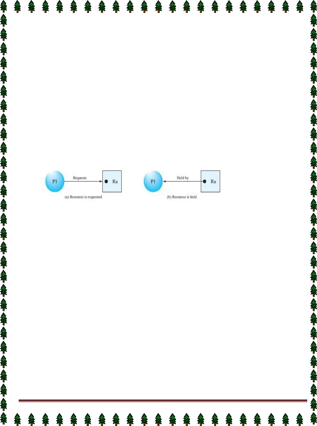
Page 45
waiting for another resource that it is holding. In addition, deadlock is not possible between two threads in a
process, because it is the process that holds resources, not the thread that is, each thread has access to the
resources held by the process.
Resource-Allocation Graph
graph.
Deadlocks can be described in terms of a directed graph called a system resource-allocation
This graph consists of a set of vertices V and a set of edges E. The set of vertices V is partitioned into
two different types of nodes P = {PI, P2, ..., Pn}, the set consisting of all the active processes in the system, and
R = {R1, R2, ..., Rm}, the set consisting of all resource types in the system.
A directed edge from process Pi to resource type Rj is denoted by PiRj; it signifies that process Pi
requested an instance of resource type Rj and is currently waiting for that resource. A directed edge Pi Rj is
called a request edge.
A directed edge from resource type Rj to process Pi is denoted by RjPi; it signifies that an instance of
resource type Rj has been allocated to process Pi. A directed edge RjPi is called an assignment edge.
Pictorially, we represent each process Pi as a circle and each resource type Rj as a square. Since
resource type Rj may have more than one instance, we represent each such instance as a dot within the square.
A request edge points to only the square Rj, whereas an assignment edge must designate one of the dots in the
square.
The resource-allocation graph shown below depicts the following situation.
The sets P, R, and E:
P={P1,P2,P3}
R={R1,R2,R3,R4}
E={P1R1, P2R3, R1P2, R2P2, R2P1, R3P3}
Resource instances:
One instance of resource type R1
Two instances of resource type R2
One instance of resource type R3
Three instances of resource type R4
Process states:
Process PI is holding an instance of resource type R2, and is waiting for an instance of resource type
R1.
Process P2 is holding an instance of R1 and R2, and is waiting for an instance of resource type R3.
Process P3 is holding an instance of R3.
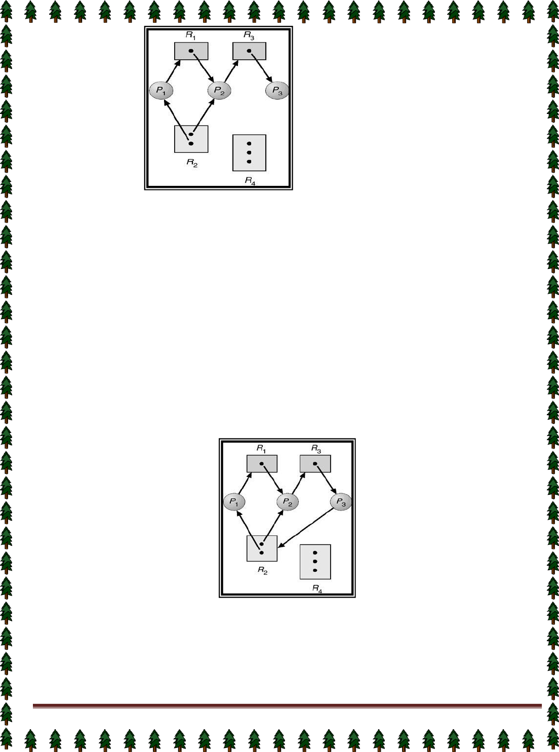
Page 46
Example of a Resource Allocation Graph
Given the definition of a resource-allocation graph, it can be shown that, if the graph contains no cycles,
then no process in the system is deadlocked. If the graph does contain a cycle, then a deadlock may exist.
If each resource type has exactly one instance, then a cycle implies that a deadlock has occurred. If the
cycle involves only a set of resource types, each of which has only a single instance, then a deadlock has
occurred. Each process involved in the cycle is deadlocked. In this case, a cycle in the graph is both a necessary
and a sufficient condition for the existence of deadlock.
If each resource type has several instances, then a cycle does not necessarily imply that a deadlock has
occurred. In this case, a cycle in the graph is a necessary but not a sufficient condition for the existence of
deadlock.
To illustrate this concept, let us return to the resource-allocation graph depicted in Figure. Suppose that
process P3 requests an instance of resource type R2. Since no resource instance is currently available, a
request edge P3 R2 is added to the graph. At this point, two minimal cycles exist in the system:
P1R1 P2 R3 P3 R2 P1
P2 R3 P3 R2 P2
Processes PI, P2, and P3 are deadlocked. Process P2 is waiting for the resource R3, which is held by process
P3. Process P3, on the other hand, is waiting for either process PI or process P2 to release resource R2. In
addition, process PI is waiting for process P2 to release resource R1.
Resource Allocation Graph with a deadlock
Now consider the resource-allocation graph in the following Figure. In this example, we also have a
cycle However, there is no deadlock. Observe that process P4 may release its instance of resource type R2.
That resource can then be allocated to P3, breaking the cycle.
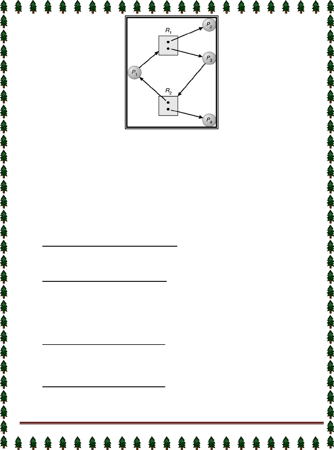
Page 47
Resource Allocation Graph with a Cycle but No Deadlock
METHODS OF HANDLING DEADLOCK
In general, there are four strategies of dealing with deadlock problem:
1.
Deadlock Prevention: Prevent deadlock by resource scheduling so as to negate at least one of the four
conditions.
2.
Deadlock Avoidance: Avoid deadlock by careful resource scheduling.
3.
Deadlock Detection and Recovery: Detect deadlock and when it occurs, take steps to recover.
4.
The Ostrich Approach: Just ignore the deadlock problem altogether.
DEADLOCK PREVENTION
A deadlock may be prevented by denying any one of the conditions.
Elimination of “Mutual Exclusion” Condition: The mutual exclusion condition must hold for non-
sharable resources. That is, several processes cannot simultaneously share a single resource. This
condition is difficult to eliminate because some resources, such as the Hard disc drive and printer, are
inherently non-shareable. Note that shareable resources like read-only-file do not require mutually
exclusive access and thus cannot be involved in deadlock.
Elimination of “Hold and Wait” Condition: There are two possibilities for elimination of the second
condition. The first alternative is that a process request be granted all of the resources it needs at once,
prior to execution. The second alternative is to disallow a process from requesting resources whenever it
has previously allocated resources. This strategy requires that all of the resources a process will need
must be requested at once. The system must grant resources on “all or none” basis. If the complete set
of resources needed by a process is not currently available, then the process must wait until the
complete set is available. While the process waits, however, it may not hold any resources. Thus the
“wait for” condition is denied and deadlocks cannot occur. This strategy can lead to serious waste of
resources.
Elimination of “No-preemption” Condition: The non-preemption condition can be alleviated by forcing
a process waiting for a resource that cannot immediately be allocated to relinquish all of its currently held
resources, so that other processes may use them to finish. This strategy requires that when a process
that is holding some resources is denied a request for additional resources. The process must release its
held resources and, if necessary, request them again together with additional resources. Implementation
of this strategy denies the “no-preemptive” condition effectively.
Elimination of “Circular Wait” Condition: The last condition, the circular wait, can be denied by
imposing a total ordering on all of the resource types and then forcing, all processes to request the
resources in order (increasing or decreasing). This strategy impose a total ordering of all resources
types, and to require that each process requests resources in a numerical order (increasing or
decreasing) of enumeration. With this rule, the resource allocation graph can never have a cycle.
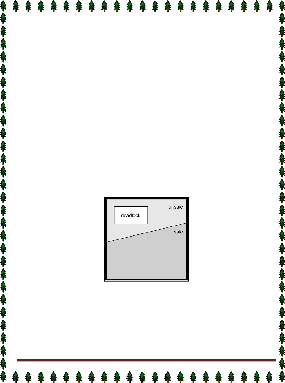
Page 48
For example, provide a global numbering of all the resources, as shown
1
≡
Card reader
2
≡
Printer
3
≡
Optical driver
4
≡
HDD
5
≡
Card punch
Now the rule is this: processes can request resources whenever they want to, but all requests must be
made in numerical order. A process may request first printer and then a HDD(order: 2, 4), but it may not
request first a optical driver and then a printer (order: 3, 2). The problem with this strategy is that it may be
impossible to find an ordering that satisfies everyone.
DEADLOCK AVOIDANCE
This approach to the deadlock problem anticipates deadlock before it actually occurs. This approach
employs an algorithm to access the possibility that deadlock could occur and acting accordingly. If the necessary
conditions for a deadlock are in place, it is still possible to avoid deadlock by being careful when resources are
allocated. It employs the most famous deadlock avoidance algorithm that is the Banker’s algorithm.
A deadlock-avoidance algorithm dynamically examines the resource-allocation state to ensure that a
circular wait condition can never exist. The resource-allocation state is defined by the number of available and
allocated resources, and the maximum demands of the processes.
Safe and Unsafe States
A system is said to be in a Safe State, if there is a safe execution sequence. An execution sequence is
an ordering for process execution such that each process runs until it terminates or blocked and all request for
resources are immediately granted if the resource is available.
A system is said to be in an Unsafe State, if there is no safe execution sequence. An unsafe state may
not be deadlocked, but there is at least one sequence of requests from processes that would make the system
deadlocked.
(Relation between Safe, Unsafe and Deadlocked States)
Resource-Allocation Graph Algorithm
The deadlock avoidance algorithm uses a variant of the resource-allocation graph to avoid deadlocked
state. It introduces a new type of edge, called a claim edge. A claim edge Pi Rj indicates that process Pi may
request resource Rj at some time in the future. This edge resembles a request edge in direction, but is
represented by a dashed line. When process Pi requests resource Rj, the claim edge Pi Rj is converted to a
request edge. Similarly, when a resource Rj is released by Pi, the assignment edge Rj Pi is reconverted to a
claim edge Pi Rj.

Page 49
Suppose that process Pi requests resource Rj. The request can be granted only if converting the request edge Pi
Rj to an assignment edge Rj Pi that does not result in the formation of a cycle in the resource-allocation
graph. An algorithm for detecting a cycle in this graph is called cycle detection algorithm.
If no cycle exists, then the allocation of the resource will leave the system in a safe state. If a cycle is
found, then the allocation will put the system in an unsafe state. Therefore, process Pi will have to wait for its
requests to be satisfied.
Banker's algorithm
The Banker's algorithm is a resource allocation & deadlock avoidance algorithm developed by Edsger
Dijkstra that test for safety by simulating the allocation of pre-determined maximum possible amounts of all
resources. Then it makes a "safe-state" check to test for possible deadlock conditions for all other pending
activities, before deciding whether allocation should be allowed to continue.
The Banker's algorithm is run by the operating system whenever a process requests resources. The
algorithm prevents deadlock by denying or postponing the request if it determines that accepting the request
could put the system in an unsafe state (one where deadlock could occur).
For the Banker's algorithm to work, it needs to know three things:
How much of each resource could possibly request by each process.
How much of each resource is currently holding by each process.
How much of each resource the system currently has available.
Resources may be allocated to a process only if it satisfies the following conditions:
1.
request ≤ max, else set error as process has crossed maximum claim made by it.
2.
request ≤ available, else process waits until resources are available.
Several data structures must be maintained to implement the banker's algorithm. These data structures
encode the state of the resource-allocation system. Let n be the number of processes in the system and m be
the number of resource types. We need the following data structures:
Available: A vector of length m indicates the number of available resources of each type. If Available[j] = k, there
are k instances of resource type Rj available.
Max: An n x m matrix defines the maximum demand of each process. If Max[i,j] = k, then process Pi may request
at most k instances of resource type Rj.
Allocation: An n x m matrix defines the number of resources of each type currently allocated to each process. If
Allocation[i,j] = k, then process Pi is currently allocated k instances of resource type Rj.
Need: An n x m matrix indicates the remaining resource need of each process. If Need[i,j] = k, then process Pi
may need k more instances of resource type Ri to complete its task. Note that Need[i,j] = Max[i,j] - Allocafion[i,j].
These data structures vary over time in both size and value. The vector Allocation
i
specifies the
resources currently allocated to process Pi; the vector Need
i
specifies the additional resources that process Pi
may still request to complete its task.
Safety Algorithm
The algorithm for finding out whether or not a system is in a safe state can be described as follows:
1.
Let Work and Finish be vectors of length m and n, respectively. Initialize
Work := Available and Finisk[i] :=false for i = 1,2, ..., n.
2.
Find an i such that both a. Finisk[i] =false
b. Need
i
< Work.
If no such i exists, go to step 4.
3.
Work := Work + Allocation
i
Finisk[i] := true
go to step 2.
4.
If Finish[i] = true for all i, then the system is in a safe state.
This algorithm may require an order of m x n
2
operations to decide whether a state is safe.

Page 50
Resource-Request Algorithm
Let Request
i
be the request vector for process Pi. If Request
i
[j] = k, then process Pi wants k instances of
resource type Rj. When a request for resources is made by process Pi, the following actions are taken:
1.
If Request
i
< Need
i
, go to step 2. Otherwise, raise an error condition, since the process has
exceeded its maximum claim.
2.
If Request
i
< Available, go to step 3. Otherwise, Pi must wait, since the resources are not
available.
3.
Have the system pretend to have allocated the requested resources to process Pi by
modifying the state as follows:
Available := Available - Request
i
;
Allocation
i
:= Allocation
i
+ Request
i
;
Need
i
:= Need
i
- Request
i
;
If the resulting resource-allocation state is safe, the transaction is completed and process Pi is allocated
its resources. However, if the new state is unsafe, then Pi must wait for Request
i
and the old resource-allocation
state is restored.
Consider a system with five processes P0 through P4 and three resource types A,B,C. Resource type A
has 10 instances, resource type B has 5 instances, and resource type C has 7 instances. Suppose that, at time
T0, the following snapshot of the system has been taken:
Allocation
------------
Max
--------
Available
-----------
A
B
C
A
B
C
A B C
P0
0
1
0
7
5
3
3 3 2
PI
2
0
0
3
2
2
P2
3
0
2
9
0
2
P3
2
1
1
2
2
2
P4
0
0
2
4
3
3
The content of the matrix Need is defined to be Max - Allocation and is
Need
We claim that the system is currently in a safe state. Indeed, the sequence <PI, P3, P4, P2, P0> satisfies the
safety criteria. Suppose now that process P1 requests one additional instance of resource type A and two
instances of resource type C, so Request1 = (1,0,2). To decide whether this request can be immediately granted,
we first check that Request1 Available (that is, (1,0,2) (3,3,2)), which is true. We then pretend that this
request has been fulfilled, and we arrive at the following new state:
Allocation
------------
Need
--------
Available
-----------
A
B
C
A
B
C
A B C
P0
0
1
0
7
4
3
2 3 0
PI
3
0
2
0
2
0
P2
3
0
2
6
0
0
P3
2
1
1
0
1
1
P4
0
0
2
4
3
1
A
B
C
P0
7
4
3
P1
1
2
2
P2
6
0
0
P3
0
1
1
P4
4
3
1
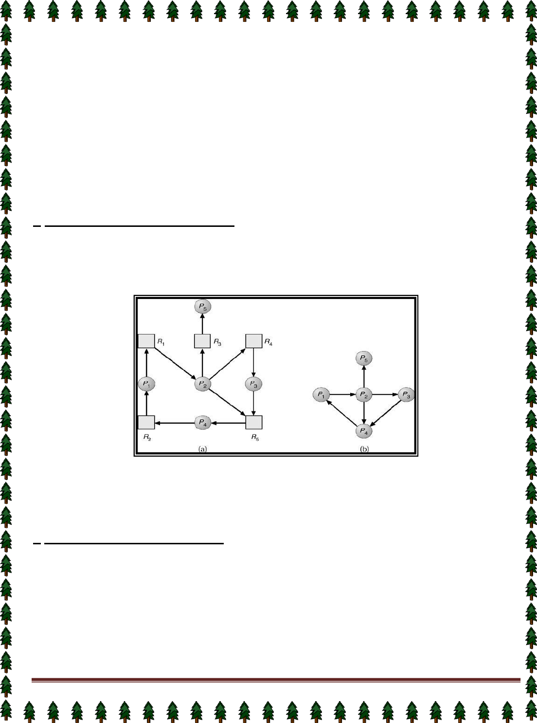
Page 51
We must determine whether this new system state is safe. To do so, we execute our safety algorithm and find
that the sequence <PI, P3, P4, P0, P2> satisfies our safety requirement. Hence, we can immediately grant the
request of process PI.
However, that when the system is in this state, a request for (3,3,0) by P4 cannot be granted, since the
resources are not available. A request for (0,2,0) by Po cannot be granted, even though the resources are
available, since the resulting state is unsafe.
DEADLOCK DETECTION
If a system does not employ either a deadlock-prevention or a deadlock avoidance algorithm, then a
deadlock situation may occur. In this environment, the system must provide:
An algorithm that examines the state of the system to determine whether a deadlock has occurred.
An algorithm to recover from the deadlock.
According to number of instances in each resource type, the Deadlock Detection algorithm can be classified into
two categories as follows:
1.
Single Instance of Each Resource Type: If all resources have only a single instance, then it can define a
deadlock detection algorithm that uses a variant of the resource-allocation graph (is called a wait-for graph). A
wait–for graph can be draw by removing the nodes of type resource and collapsing the appropriate edges from
the resource-allocation graph.
An edge from Pi to Pj in a wait-for graph implies that process Pi is waiting for process Pj to release a
resource that Pi needs. An edge Pi Pj exists in a wait-for graph if and only if the corresponding resource
allocation graph contains two edges Pi Rq and Rq Pj for some resource Rq. For Example:
((a) Resource-allocation graph. (b) Corresponding wait-for graph)
A deadlock exists in the system if and only if the wait-for graph contains a cycle. To detect deadlocks,
the system needs to maintain the wait-for graph and periodically to invoke an algorithm that searches for a cycle
in the graph. An algorithm to detect a cycle in a graph requires an order of n
2
operations, where n is the number
of vertices in the graph.
2.
Several Instances of a Resource Type: The following deadlock-detection algorithm is applicable to several
instance of a resource type. The algorithm employs several time-varying data structures:
Available: A vector of length m indicates the number of available resources of each type.
Allocation: An n x m matrix defines the number of resources of each type currently allocated to each process.
Request: An n x m matrix indicates the current request of each process. If Request[i,j] = k, then process Pi is
requesting k more instances of resource type Rj.
The detection algorithm is described as follows:
1.
Let Work and Finish be vectors of length m and n, respectively.
Initialize, Work := Available. For i = 1, 2, ..., n,
if Allocation
i
!= 0, then Finish[i] :=false; otherwise, Finish[i] := true.
2.
Find an index i such that both
a.
Finish[i] =false.

Page 52
state.
b.
Request
i
< Work.
If no such i exists, go to step 4.
3.
Work := Work + Allocation
i
Finish[i] := true
go to step 2.
4.
If Finish[i] = false, for some i, 1 < i < n, then the system is in a deadlock state.
if Finish[i] =false, then process Pi is deadlocked.
This algorithm requires an order of m x n
2
operations to detect whether the system is in a deadlocked
RECOVERY FROM DEADLOCK
When a detection algorithm determines that a deadlock exists, then the system or operator is
responsible for handling deadlock problem. There are two options for breaking a deadlock.
1.
Process Termination
2.
Resource preemption
3.
Process Termination
There are two method to eliminate deadlocks by terminating a process as follows:
1.
Abort all deadlocked processes: This method will break the deadlock cycle clearly by terminating all
process. This method is cost effective. And it removes the partial computations completed by the processes.
2.
Abort one process at a time until the deadlock cycle is eliminated: This method terminates one process
at a time, and invokes a deadlock-detection algorithm to determine whether any processes are still
deadlocked.
Resource Preemption
In resource preemption, the operator or system preempts some resources from processes and give
these resources to other processes until the deadlock cycle is broken.
If preemption is required to deal with deadlocks, then three issues need to be addressed:
1.
Selecting a victim: The system or operator selects which resources and which processes are to be
preempted based on cost factor.
2.
Rollback: The system or operator must roll back the process to some safe state and restart it from that
state.
3.
Starvation: The system or operator should ensure that resources will not always be preempted from the
same process?
MEMORY MANAGEMENT
In a uni-programming system, main memory is divided into two parts: one part for the
operating system (resident monitor, kernel) and one part for the user program currently being
executed.
In a multiprogramming system, the “user” part of memory must be further subdivided
to accommodate multiple processes. The task of subdivision is carried out dynamically by the
operating system and is known as
memory management
.
Binding of Instructions and Data to Memory
Address binding of instructions and data to memory addresses can happen at three different
stages.
1.
Compile time
: The compile time is the time taken to compile the program or source code.
During compilation, if memory location known a priori, then it generates absolute codes.
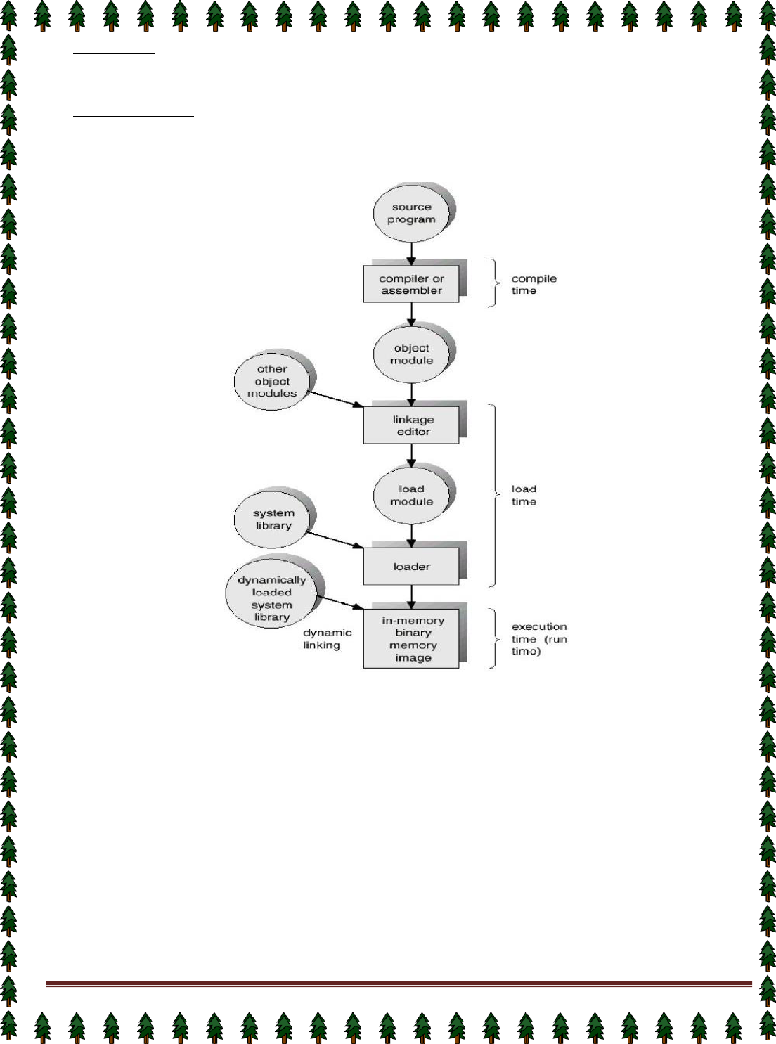
Page 53
2.
Load time: It is the time taken to link all related program file and load into the main
memory. It must generate relocatable code if memory location is not known at compile
time.
3.
Execution time
: It is the time taken to execute the program in main memory by processor.
Binding delayed until run time if the process can be moved during its execution from one
memory segment to another. Need hardware support for address maps (e.g., base and
limit registers).
(Multistep processing of a user program.)
Logical- Versus Physical-Address Space
An address generated by the CPU is commonly referred to as a logical address or a
virtual address whereas an address seen by the main memory unit is commonly referred
to as a physical address.
The set of all logical addresses generated by a program is a logical-address space whereas
the set of all physical addresses corresponding to these logical addresses is a physical-
address space.
Logical and physical addresses are the same in compile-time and load-time address-
binding schemes; logical (virtual) and physical addresses differ in execution-time address-
binding scheme.
The Memory Management Unit is a hardware device that maps virtual to physical
address. In MMU scheme, the value in the relocation register is added to every address
generated by a user process at the time it is sent to memory as follows:
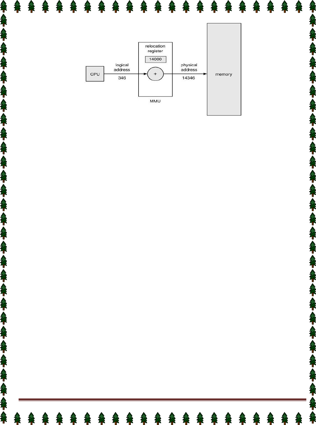
Page 54
(Dynamic relocation using a relocation register
)
Dynamic Loading
It loads the program and data dynamically into physical memory to obtain better
memory-space utilization.
With dynamic loading, a routine is not loaded until it is called.
The advantage of dynamic loading is that an unused routine is never loaded.
This method is useful when large amounts of code are needed to handle infrequently
occurring cases, such as error routines.
Dynamic loading does not require special support from the operating system.
Dynamic Linking
Linking postponed until execution time.
Small piece of code (stub) used to locate the appropriate memory-resident library routine.
Stub replaces itself with the address of the routine and executes the routine.
Operating system needed to check if routine is in processes memory address.
Dynamic linking is particularly useful for libraries.
Overlays
Keep in memory only those instructions and data that are needed at any given time.
Needed when process is larger than amount of memory allocated to it.
Implemented by user, no special support needed from operating system, programming
design of overlay structure is complex.
Swapping
A process can be swapped temporarily out of memory to a backing store (large disc), and
then brought back into memory for continued execution.
Roll out, roll in
: A variant of this swapping policy is used for priority-based scheduling
algorithms. If a higher-priority process arrives and wants service, the memory manager
can swap out the lower-priority process so that it can load and execute the higher-priority
process. When the higher-priority process finishes, the lower-priority process can be
swapped back in and continued. This variant of swapping is called
roll out, roll in.
Major part of swap time is transfer time; total transfer time is directly proportional to the
amount of memory swapped.
Modified versions of swapping are found on many systems (UNIX, Linux, and Windows).
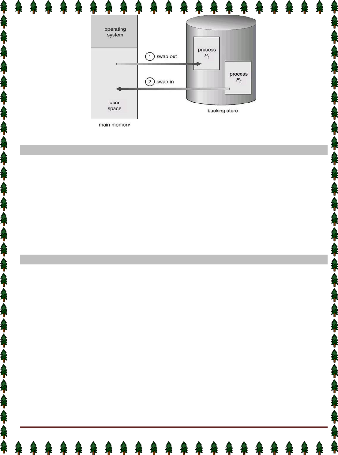
Page 55
(Schematic View of Swapping)
The main memory must accommodate both the operating system and the various user
processes. We need to allocate different parts of the main memory in the most efficient way
possible.
The main memory is usually divided into two partitions: one for the resident operating
system, and one for the user processes. We may place the operating system in either low
memory or high memory. The major factor affecting this decision is the location of the
interrupt vector. Since the interrupt vector is often in low memory, programmers usually
place the operating system in low memory as well.
There are following two ways to allocate memory for user processes:
1.
Contiguous memory allocation
2.
Non contiguous memory allocation
Here, all the processes are stored in contiguous memory locations. To load multiple
processes into memory, the Operating System must divide memory into multiple partitions
for those processes.
Hardware Support: The relocation-register scheme used to protect user processes from each
other, and from changing operating system code and data. Relocation register contains value
of smallest physical address of a partition and limit register contains range of that partition.
Each logical address must be less than the limit register.
MEMORY ALLOCATION
1. Contiguous Memory Allocation
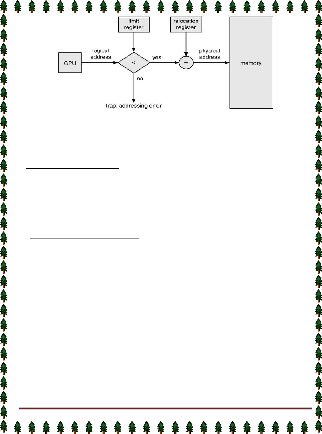
Page 56
(Hardware support for relocation and limit registers)
According to size of partitions, the multiple partition schemes are divided into two types:
i.
Multiple fixed partition/ multiprogramming with fixed task(MFT)
ii.
Multiple variable partition/ multiprogramming with variable task(MVT)
i.
Multiple fixed partitions: Main memory is divided into a number of static partitions at
system generation time. In this case, any process whose size is less than or equal to the
partition size can be loaded into any available partition. If all partitions are full and no
process is in the Ready or Running state, the operating system can swap a process out of any
of the partitions and load in another process, so that there is some work for the processor.
Advantages:
Simple to implement and little operating system overhead.
Disadvantage: *
Inefficient use of memory due to internal fragmentation.
* Maximum number of active processes is fixed.
ii.
Multiple variable partitions:
With this partitioning, the partitions are of variable
length and number. When a process is brought into main memory, it is allocated exactly as
much memory as it requires and no more.
Advantages:
No internal fragmentation and more efficient use of main memory.
Disadvantages: Inefficient use of processor due to the need for compaction to counter
external fragmentation.
Partition Selection policy:
When the multiple memory holes (partitions) are large enough to contain a process, the
operating system must use an algorithm to select in which hole the process will be loaded.
The partition selection algorithm are as follows:
First-fit
: The OS looks at all sections of free memory. The process is allocated to the first
hole found that is big enough size than the size of process.
Next Fit: The next fit search starts at the last hole allocated and The process is allocated to
the next hole found that is big enough size than the size of process.
Best-fit: The Best Fit searches the entire list of holes to find the smallest hole that is big
enough size than the size of process.
Worst-fit: The Worst Fit searches the entire list of holes to find the largest hole that is big
enough size than the size of process.
Fragmentation: The wasting of memory space is called fragmentation. There are two types
of fragmentation as follows:
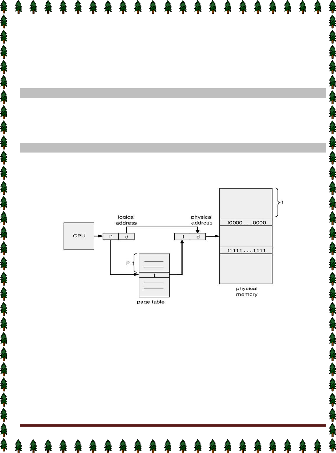
Page 57
1.
External Fragmentation:
The total memory space exists to satisfy a request, but it is not
contiguous. This wasted space not allocated to any partition is called external
fragmentation. The external fragmentation can be reduce by compaction. The goal is to
shuffle the memory contents to place all free memory together in one large block.
Compaction is possible only if relocation is dynamic, and is done at execution time.
2.
Internal Fragmentation:
The allocated memory may be slightly larger than requested
memory. The wasted space within a partition is called internal fragmentation. One
method to reduce internal fragmentation is to use partitions of different size.
In noncontiguous memory allocation, it is allowed to store the processes in non
contiguous memory locations. There are different techniques used to load processes into
memory, as follows:
1.
Paging
2.
Segmentation
3.
Virtual memory paging(Demand
paging) etc.
Main memory is divided into a number of equal-size blocks, are called
frames
. Each
process is divided into a number of equal-size block of the same length as frames, are called
Pages
. A process is loaded by loading all of its pages into available frames (may not be
contiguous).
(Diagram of Paging hardware)
Process of Translation from logical to physical addresses
Every address generated by the CPU is divided into two parts: a page number (p) and a
page offset (d). The page number is used as an index into a page table.
The page table contains the base address of each page in physical memory. This base
address is combined with the page offset to define the physical memory address that is
sent to the memory unit.
If the size of logical-address space is 2
m
and a page size is
2
n
addressing units (bytes or
words), then the high-order (m – n) bits of a logical address designate the page number
and the n low-order bits designate the page offset. Thus, the logical address is as follows:
PAGING
2. Noncontiguous memory allocation
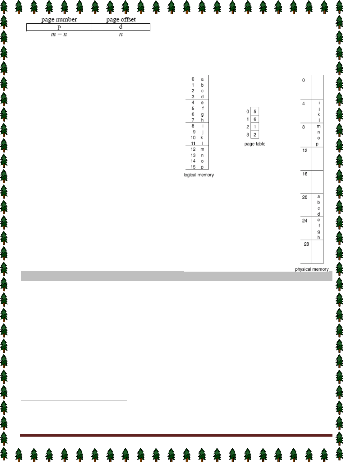
Page 58
Where p is an index into the page table and d is the displacement within the page.
Example:
Consider a page size of 4 bytes and a
physical memory of 32 bytes (8 pages), we
show how the user's view of memory can
be mapped into physical memory. Logical
address 0 is page 0, offset 0. Indexing into
the page table, we find that page 0 is in
frame 5. Thus, logical address 0 maps to
physical address 20 (= (5 x 4) + 0). Logical
address 3 (page 0, offset 3) maps to
physical address 23 (= (5 x 4) + 3). Logical
address 4 is page 1, offset 0; according to
the page table, page 1 is mapped to frame
6. Thus, logical address 4 maps to physical
address 24 (= (6 x 4) + 0). Logical address
13 maps to physical address 9(= (2 x 4)+1).
Hardware Support for Paging:
Each operating system has its own methods for storing page tables. Most operating
systems allocate a page table for each process. A pointer to the page table is stored with the
other register values (like the instruction counter) in the process control block. When the
dispatcher is told to start a process, it must reload the user registers and define the correct
hardware page table values from the stored user page table.
Implementation of Page Table
Generally, Page table is kept in main memory. The Page Table Base Register (PTBR) points
to the page table. And Page-table length register (PRLR) indicates size of the page table.
In this scheme every data/instruction access requires two memory accesses. One for the
page table and one for the data/instruction.
The two memory access problem can be solved by the use of a special fast-lookup
hardware cache called associative memory or translation look-aside buffers (TLBs).
Paging Hardware With TLB
The TLB is an associative and high-speed memory. Each entry in the TLB consists of two
parts: a key (or tag) and a value. The TLB is used with page tables in the following way.
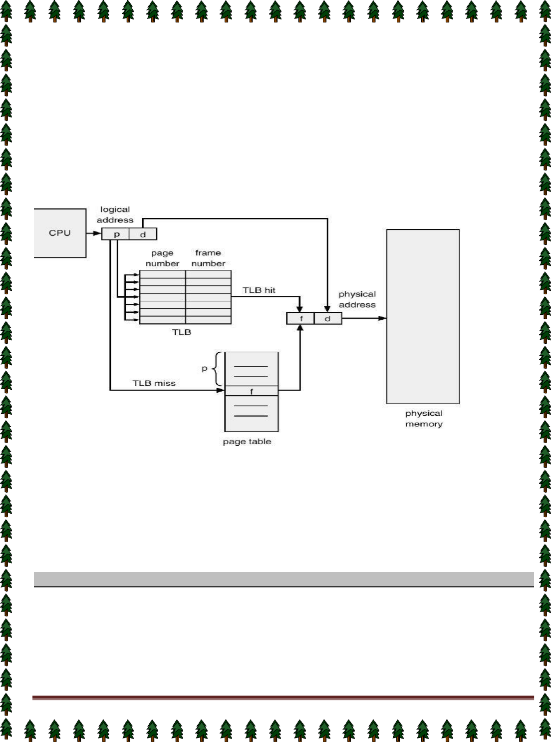
Page 59
The TLB contains only a few of the page-table entries. When a logical address is generated
by the CPU, its page number is presented to the TLB.
If the page number is found (known as a
TLB Hit
), its frame number is immediately
available and is used to access memory. It takes only one memory access.
If the page number is not in the TLB (known as a TLB miss), a memory reference to the
page table must be made. When the frame number is obtained, we can use it to access
memory. It takes two memory accesses.
In addition, it stores the page number and frame number to the TLB, so that they will be
found quickly on the next reference.
If the TLB is already full of entries, the operating system must select one for replacement
by using replacement algorithm.
(Paging hardware with TLB)
The percentage of times that a particular page number is found in the TLB is called the
hit ratio. The effective access time (EAT) is obtained as follows:
EAT= HR x (TLBAT + MAT) + MR x (TLBAT + 2 x MAT)
Where HR: Hit Ratio, TLBAT: TLB access time, MAT: Memory access time, MR: Miss Ratio.
Memory protection in Paged Environment:
Memory protection in a paged environment is accomplished by protection bits that are
associated with each frame. These bits are kept in the page table.
One bit can define a page to be read-write or read-only. This protection bit can be checked
to verify that no writes are being made to a read-only page. An attempt to write to a read-
only page causes a hardware trap to the operating system (or memory-protection
violation).
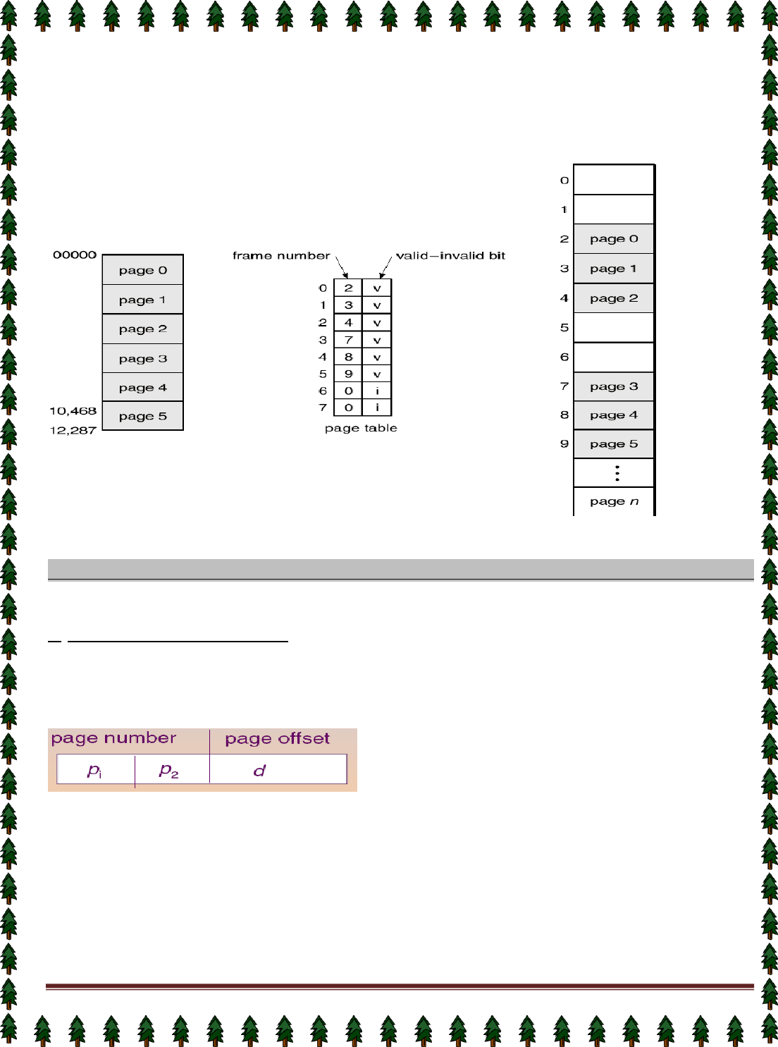
Page 60
One more bit is attached to each entry in the page table: a
valid-invalid
bit. When this bit
is set to "valid," this value indicates that the associated page is in the process' logical-
address space, and is a legal (or valid) page. If the bit is set to "invalid," this value indicates
that the page is not in the process' logical-address space.
Illegal addresses are trapped by using the valid-invalid bit. The operating system sets this
bit for each page to allow or disallow accesses to that page.
(Valid (v) or invalid (i) bit in a page table)
Structure of the Page Table
There are different structures of page table described as follows:
1.
Hierarchical Page table: When the number of pages is very high, then the page table
takes large amount of memory space. In such cases, we use multilevel paging scheme for
reducing size of page table. A simple technique is a two-level page table. Since the page table
is paged, the page number is further divided into parts: page number and page offset. Thus,
a logical address is as follows:
Where p
i
is an index into the outer page table, and p2 is the displacement within the page of
the outer page table.
Two-Level Page-Table Scheme:
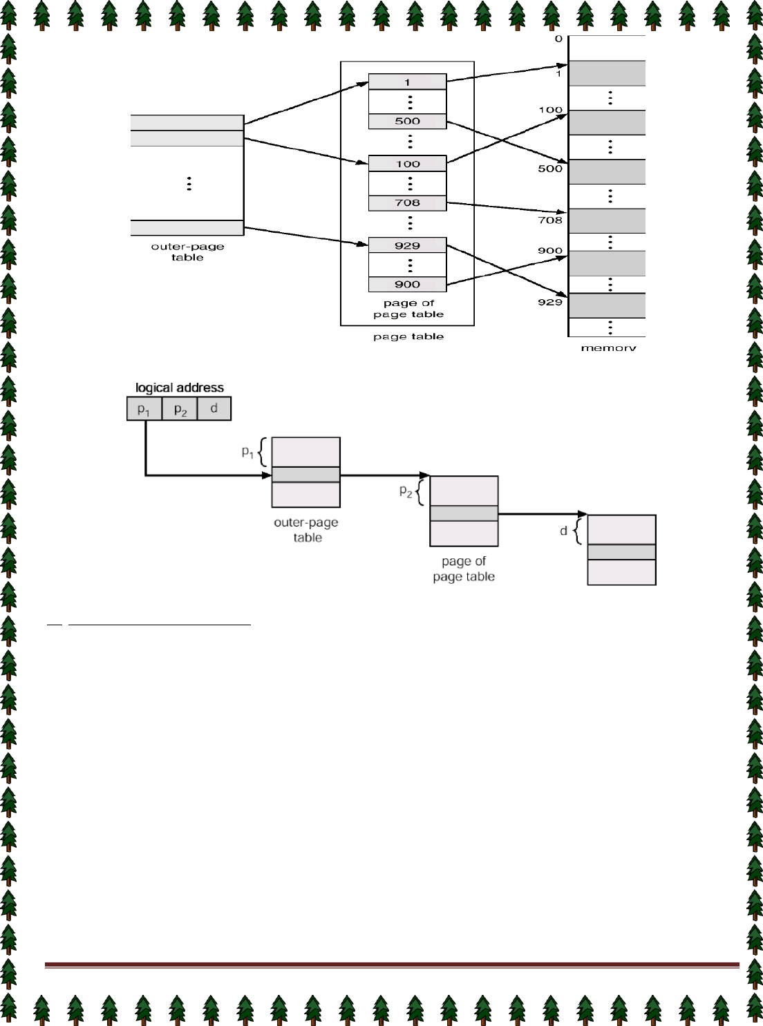
Page 61
Address translation scheme for a two-level paging architecture:
2.
Hashed Page Tables:
This scheme is applicable for address space larger than 32bits. In
this scheme, the virtual page number is hashed into a page table. This page table contains a
chain of elements hashing to the same location. Virtual page numbers are compared in this
chain searching for a match. If a match is found, the corresponding physical frame is
extracted.
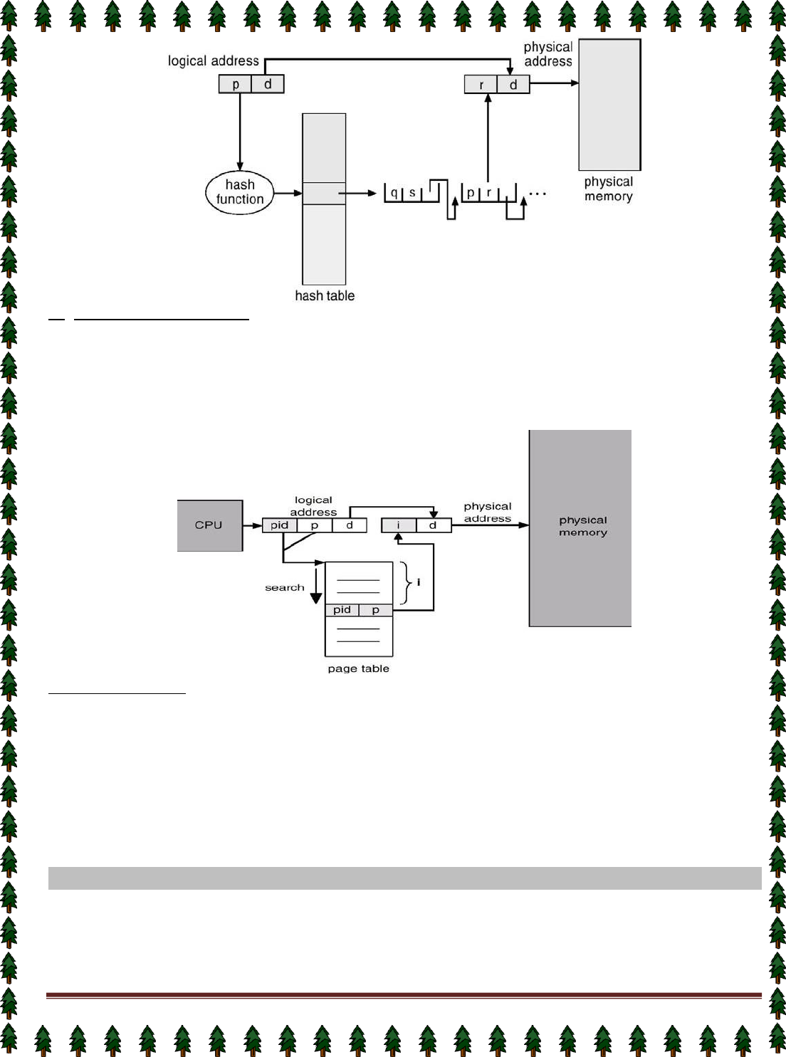
Page 62
3.
Inverted Page Table:
One entry for each real page of memory.
Entry consists of the virtual address of the page stored in that real memory location, with
information about the process that owns that page.
Decreases memory needed to store each page table, but increases time needed to search
the table when a page reference occurs.
Shared Pages
Shared code
One copy of read-only (reentrant) code shared among processes (i.e., text editors,
compilers, window systems).
Shared code must appear in same location in the logical address space of all processes.
Private code and data
Each process keeps a separate copy of the code and data.
The pages for the private code and data can appear anywhere in the logical address space.
SEGMENTATION
Segmentation is a memory-management scheme that supports user view of memory. A
program is a collection of segments. A segment is a logical unit such as: main program,
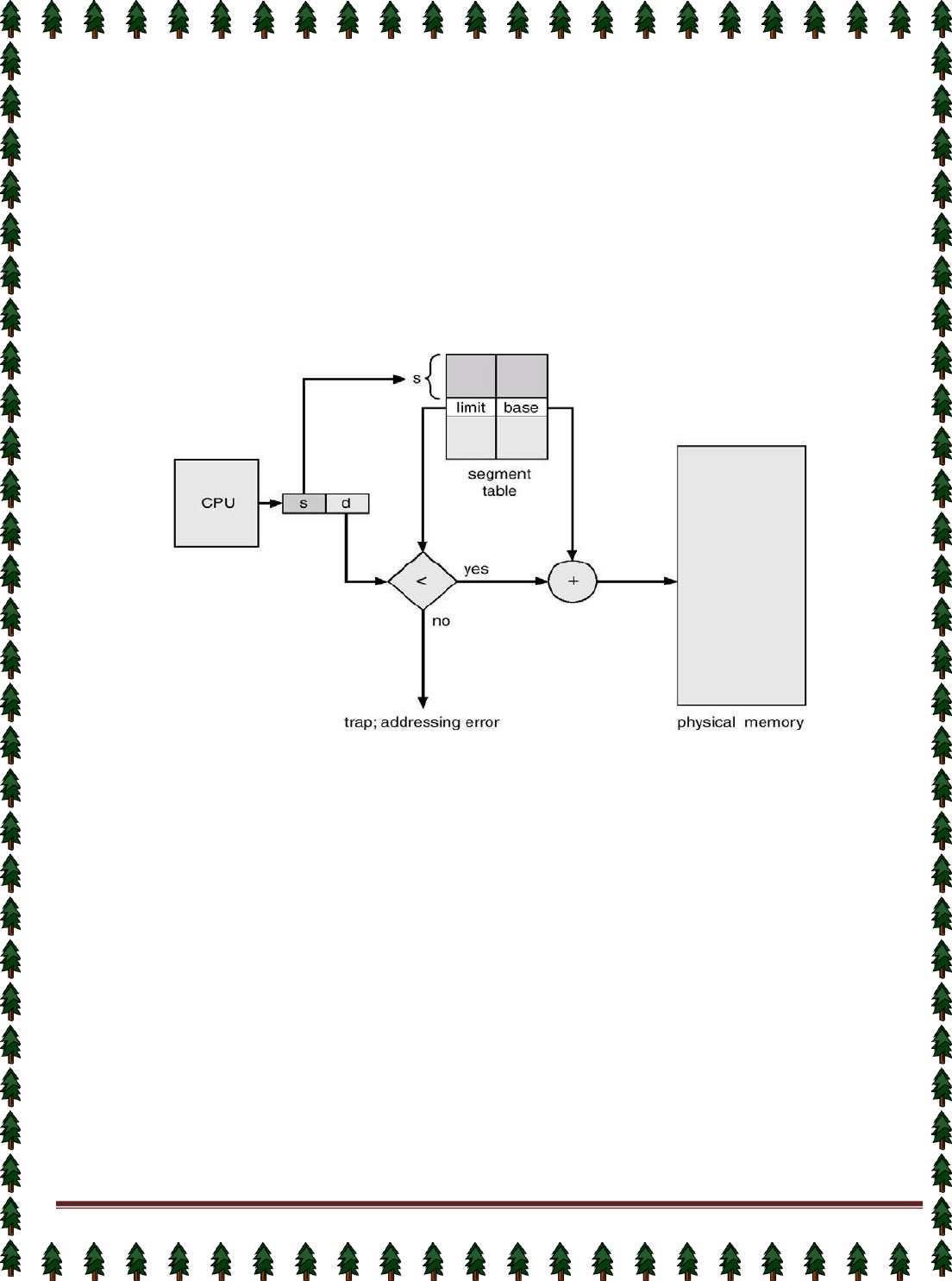
Page 63
procedure, function, method, object, local variables, global variables, common block, stack,
symbol table, arrays etc.
A logical-address space is a collection of segments. Each segment has a name and a
length. The user specifies each address by two quantities: a segment name/number and an
offset.
Hence, Logical address consists of a two tuple: <segment-number, offset>
Segment table maps two-dimensional physical addresses and each entry in table has:
base
– contains the starting physical address where the segments reside in memory.
limit
– specifies the length of the segment.
Segment-table base register (STBR) points to the segment table’s location in memory.
Segment-table length register (STLR) indicates number of segments used by a program.
(Diagram of Segmentation Hardware)
The segment number is used as an index into the segment table. The offset d of the
logical address must be between 0 and the segment limit. If it is not, we trap to the operating
system that logical addressing attempt beyond end of segment. If this offset is legal, it is
added to the segment base to produce the address in physical memory of the desired byte.
Consider we have five segments numbered from 0 through 4. The segments are stored
in physical memory as shown in figure. The segment table has a separate entry for each
segment, giving start address in physical memory (or base) and the length of that segment
(or limit). For example, segment 2 is 400 bytes long and begins at location 4300. Thus, a
reference to byte 53 of segment 2 is mapped onto location 4300 + 53 = 4353.
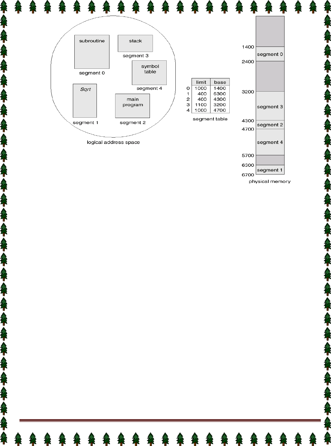
Page 64
(Example of segmentation)
VIRTUAL MEMORY
Virtual memory is a technique that allows the execution of processes that may not be
completely in memory. Only part of the program needs to be in memory for execution. It
means that Logical address space can be much larger than physical address space. Virtual
memory allows processes to easily share files and address spaces, and it provides an efficient
mechanism for process creation.
Virtual memory is the separation of user logical memory from physical memory. This
separation allows an extremely large virtual memory to be provided for programmers when
only a smaller physical memory is available. Virtual memory makes the task of programming
much easier, because the programmer no longer needs to worry about the amount of physical
memory available.
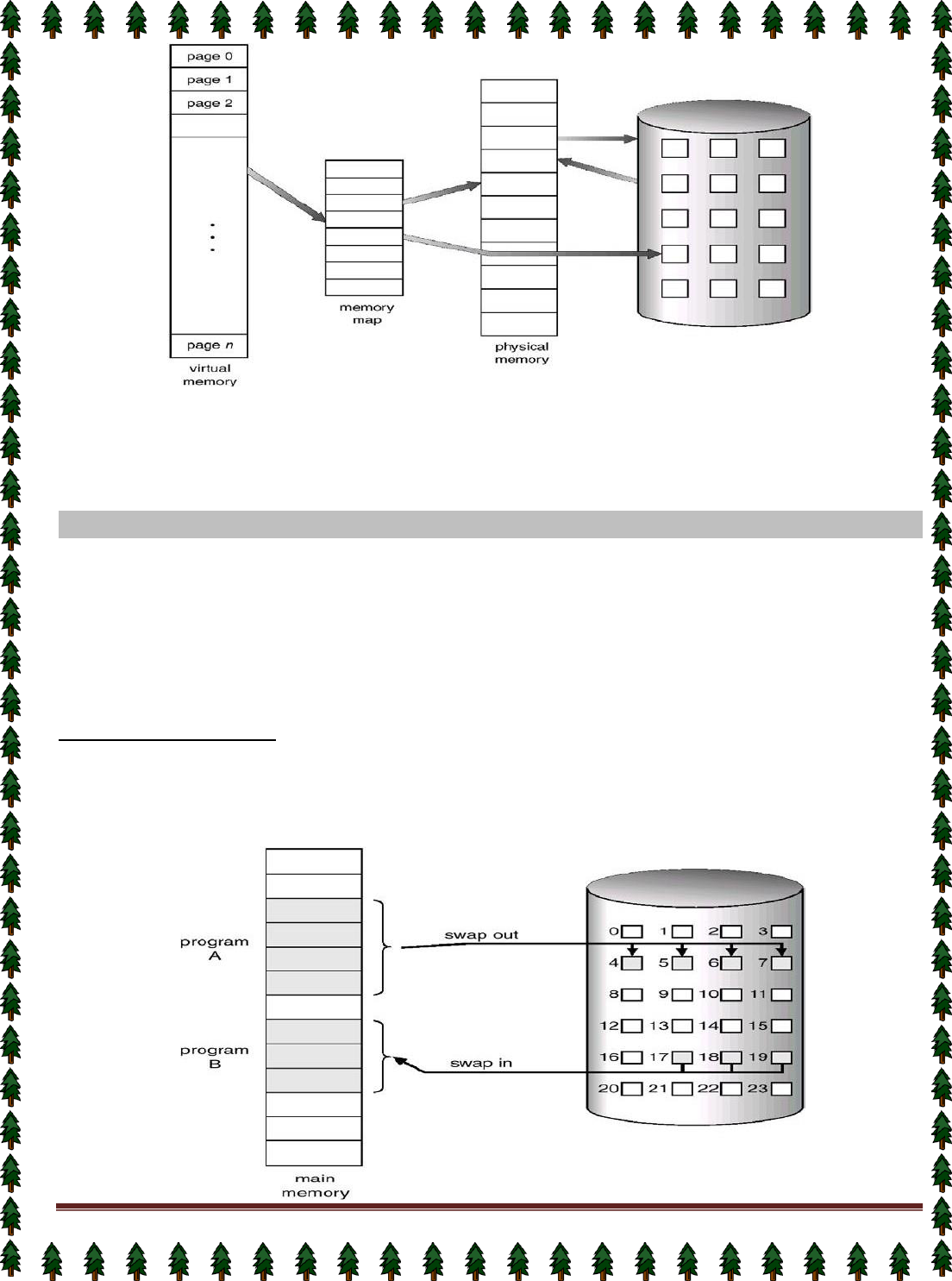
Page 65
(Diagram showing virtual memory that is larger than physical memory)
Virtual memory can be implemented via:
Demand paging
Demand segmentation
DEMAND PAGING
A demand-paging system is similar to a paging system with swapping. Generally,
Processes reside on secondary memory (which is usually a disk). When we want to execute a
process, we swap it into memory. Rather than swapping the entire process into memory, it
swaps the required page. This can be done by a
lazy swapper.
A lazy swapper never swaps a page into memory unless that page will be needed. A
swapper manipulates entire processes, whereas a
pager
is concerned with the individual
pages of a process.
Page transfer Method: When a process is to be swapped in, the pager guesses which pages
will be used before the process is swapped out again. Instead of swapping in a whole process,
the pager brings only those necessary pages into memory. Thus, it avoids reading into
memory pages that will not be used anyway, decreasing the swap time and the amount of
physical memory needed.
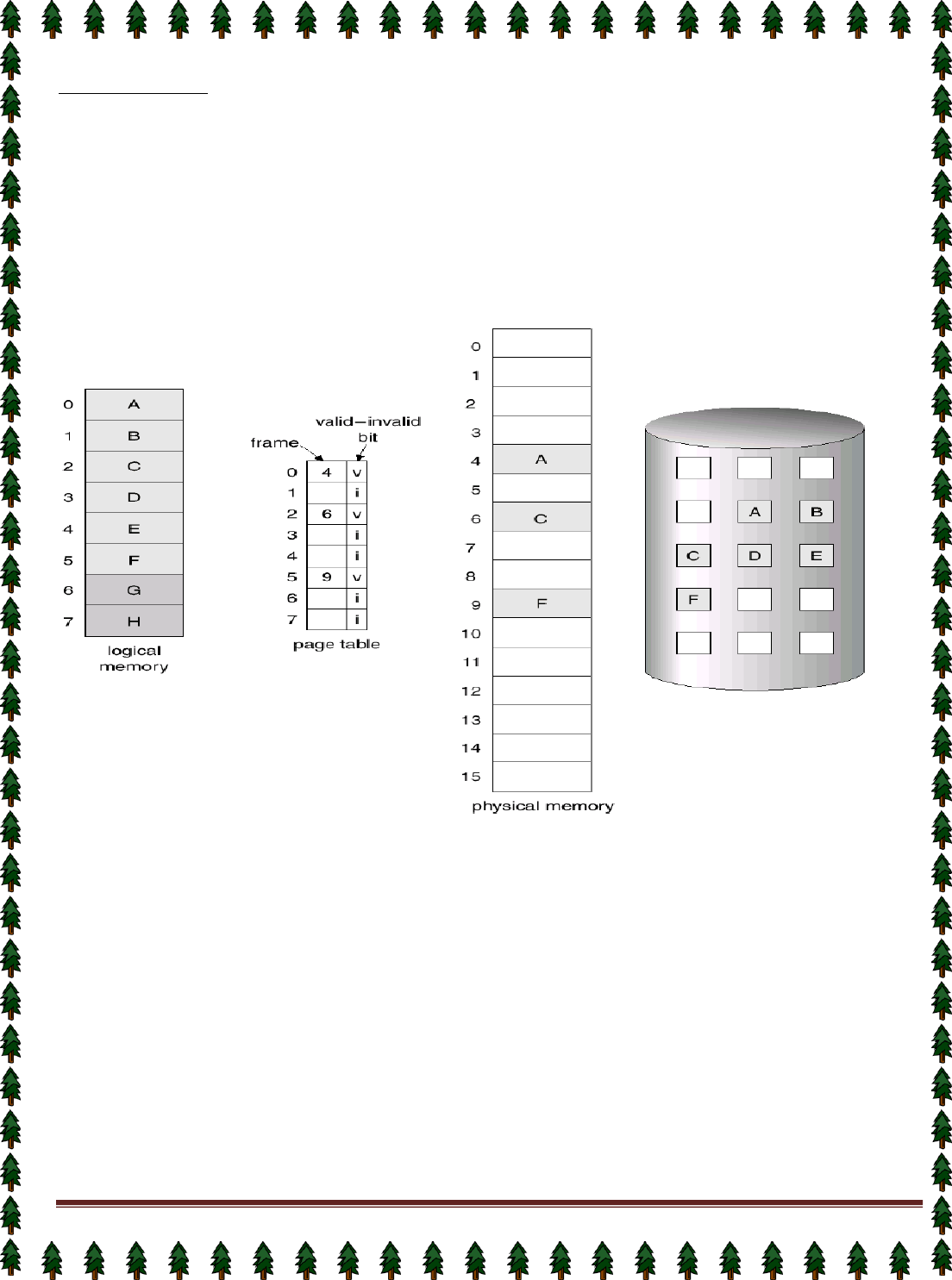
Page 66
(Transfer of a paged memory to contiguous disk space)
Page Table:
The valid-invalid bit scheme of Page table can be used for indicating which pages are
currently in memory.
When this bit is set to "valid", this value indicates that the associated page is both legal and
in memory. If the bit is set to "invalid", this value indicates that the page either is not valid
or is valid but is currently on the disk.
The page-table entry for a page that is brought into memory is set as usual, but the page-
table entry for a page that is not currently in memory is simply marked invalid, or
contains the address of the page on disk.
(Page table when some pages are not in main memory)
When a page references an invalid page, then it is called Page Fault. It means that page is
not in main memory. The procedure for handling page fault is as follows:
1.
We check an internal table for this process, to determine whether the reference was a
valid or invalid memory access.
2.
If the reference was invalid, we terminate the process. If it was valid, but we have not
yet brought in that page in to memory.
3.
We find a free frame (by taking one from the free-frame list).
4.
We schedule a disk operation to read the desired page into the newly allocated frame.
5.
When the disk read is complete, we modify the internal table kept with the process and
the page table to indicate that the page is now in memory.
6.
We restart the instruction that was interrupted by the illegal address trap. The process
can now access the page as though it had always been in memory.
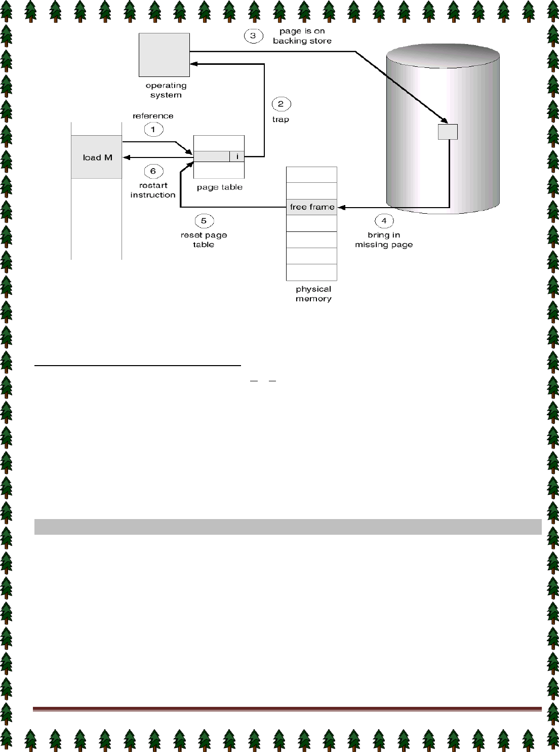
Page 67
(Diagram of Steps in handling a page fault)
Note:
The pages are copied into memory, only when they are required. This mechanism is
called
Pure Demand Paging
.
Performance of Demand Paging
Let p be the probability of a page fault (0< p < 1). Then the
effective access time
is
Effective access time = (1 - p) x memory access time + p x page fault time
In any case, we are faced with three major components of the page-fault service time:
1.
Service the page-fault interrupt.
2.
Read in the page.
3.
Restart the process.
PAGE REPLACEMENT
The page replacement is a mechanism that loads a page from disc to memory when a
page of memory needs to be allocated. Page replacement can be described as follows:
1.
Find the location of the desired page on the disk.
2.
Find a free frame:
a.
If there is a free frame, use it.
b.
If there is no free frame, use a page-replacement algorithm to select a victim frame.
c.
Write the victim page to the disk; change the page and frame tables accordingly.
3.
Read the desired page into the (newly) free frame; change the page and frame tables.
4.
Restart the user process.
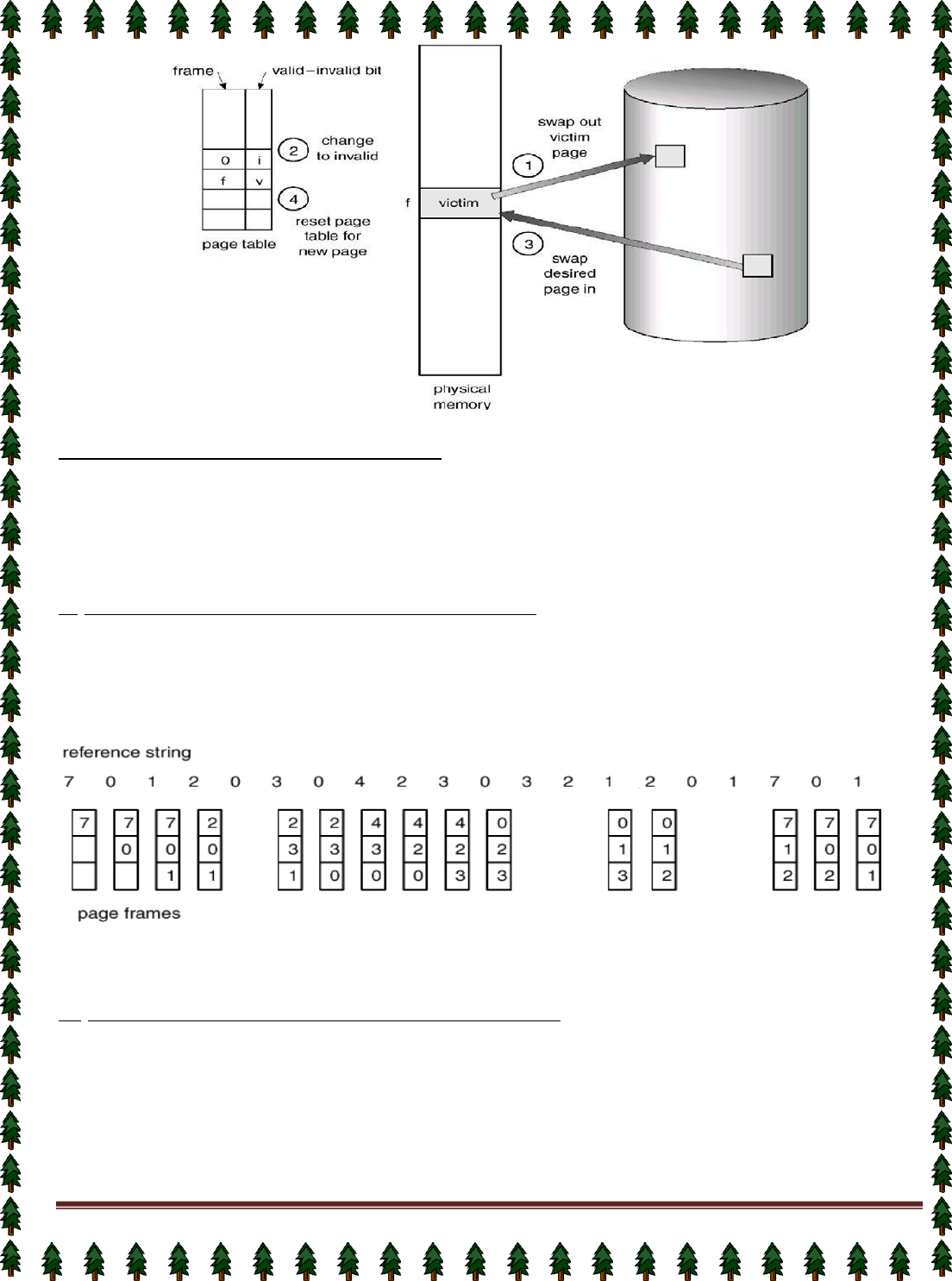
Page 68
(Diagram of Page replacement)
Page Replacement Algorithms: The page replacement algorithms decide which
memory pages to page out (swap out, write to disk) when a page of memory needs to be
allocated. We evaluate an algorithm by running it on a particular string of memory references
and computing the number of page faults. The string of memory references is called a
reference string.
The different page replacement algorithms are described as follows:
1. First-In-First-Out (FIFO) Algorithm:
A FIFO replacement algorithm associates with each page the time when that page was
brought into memory. When a page must be replaced, the oldest page is chosen to swap out.
We can create a FIFO queue to hold all pages in memory. We replace the page at the head of
the queue. When a page is brought into memory, we insert it at the tail of the queue.
Example:
(FIFO page-replacement algorithm)
Note: For some page-replacement algorithms, the page fault rate may increase as the number
of allocated frames increases. This most unexpected result is known as Belady's anomaly.
2. Optimal Page Replacement algorithm:
One result of the discovery of Belady's anomaly was the search for an
optimal page
replacement algorithm.
An optimal page-replacement algorithm has the lowest page-fault
rate of all algorithms, and will never suffer from Belady's anomaly. Such an algorithm does
exist, and has been called OPT or MIN.

Page 69
It is simply “Replace the page that will not be used for the longest period of time”. Use
of this page-replacement algorithm guarantees the lowest possible pagefault rate for a fixed
number of frames.
Example:
(Optimal page-replacement algorithm)
3. LRU Page Replacement algorithm
If we use the recent past as an approximation of the near future, then we will replace
the page that has not been used for the longest period of time. This approach is the
least-
recently-used (LRU)
algorithm.
LRU replacement associates with each page the time of that page's last use. When a
page must be replaced, LRU chooses that page that has not been used for the longest period
of time.
Example:
(LRU page-replacement algorithm)
The major problem is
how
to implement LRU replacement. An LRU page-replacement
algorithm may require substantial hardware assistance. The problem is to determine an order
for the frames defined by the time of last use. Two implementations are feasible:
Counters:
We associate with each page-table entry a time-of-use field, and add to the CPU a
logical clock or counter. The clock is incremented for every memory reference. Whenever a
reference to a page is made, the contents of the clock register are copied to the time-of-use
field in the page-table entry for that page. We replace the page with the smallest time value.
This scheme requires a search of the page table to find the LRU page, and a write to memory
(to the time-of-use field in the page table) for each memory access. The times must also be
maintained when page tables are changed (due to CPU scheduling).
Stack:
Another approach to implementing LRU replacement is to keep a stack of page
numbers. Whenever a page is referenced, it is removed from the stack and put on the top. In
this way, the top of the stack is always the most recently used page and the bottom is the LRU
page. Because entries must be removed from the middle of the stack, it is best implemented
by a doubly linked list, with a head and tail pointer. Each update is a little more expensive,
but there is no search for a replacement; the tail pointer points to the bottom of the stack,

Page 70
which is the LRU page. This approach is particularly appropriate for software or microcode
impleme-ntations of LRU replacement. Example:
(Use of a stack to record the most recent page references)
4. LRU Approximation Page Replacement algorithm
In this algorithm, Reference bits are associated with each entry in the page table.
Initially, all bits are cleared (to 0) by the operating system. As a user process executes, the bit
associated with each page referenced is set (to 1) by the hardware. After some time, we can
determine which pages have been used and which have not been used by examining the
reference bits.
This algorithm can be classified into different categories as follows:
i.
Additional-Reference-Bits Algorithm: It can keep an 8-bit(1 byte) for each page
in a page table in memory. At regular intervals, a timer interrupt transfers control to the
operating system. The operating system shifts the reference bit for each page into the high-
order bit of its 8-bit, shifting the other bits right over 1 bit position, discarding the low-order
bit. These 8 bits shift registers contain the history of page use for the last eight time periods.
If we interpret these 8-bits as unsigned integers, the page with the lowest number is the
LRU page, and it can be replaced.
ii.
Second-Chance Algorithm: The basic algorithm of second-chance replacement is
a FIFO replacement algorithm. When a page has been selected, we inspect its reference bit.
If the value is 0, we proceed to replace this page. If the reference bit is set to 1, we give that
page a second chance and move on to select the next FIFO page. When a page gets a second
chance, its reference bit is cleared and its arrival time is reset to the current time. Thus, a
page that is given a second chance will not be replaced until all other pages are replaced.
5. Counting-Based Page Replacement
We could keep a counter of the number of references that have been made to each
page, and develop the following two schemes.
i.
LFU page replacement algorithm: The least frequently used (LFU) page-
replacement algorithm requires that the page with the smallest count be replaced. The
reason for this selection is that an actively used page should have a large reference count.
ii.
MFU page-replacement algorithm: The most frequently used (MFU) page
replacement algorithm is based on the argument that the page with the largest count be
replaced.
ALLOCATION OF FRAMES
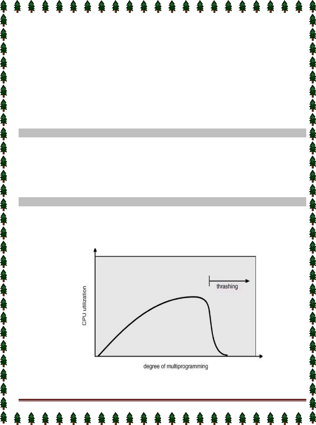
Page 71
When a page fault occurs, there is a free frame available to store new page into a frame.
While the page swap is taking place, a replacement can be selected, which is written to the
disk as the user process continues to execute. The operating system allocate all its buffer and
table space from the free-frame list for new page.
Two major allocation Algorithm/schemes.
1.
equal allocation
2.
proportional allocation
1.
Equal allocation: The easiest way to split m frames among n processes is to give
everyone an equal share, m/n frames. This scheme is called equal allocation.
2.
proportional allocation: Here, it allocates available memory to each process according
to its size. Let the size of the virtual memory for process p
i
be s
i
, and define S= ∑ Si
Then, if the total number of available frames is
m,
we allocate
a
i
frames to process
p
i
, where
a
i
is approximately
a
i
=
Si/ S x m.
We can classify page-replacement algorithms into two broad categories: global
replacement and local replacement.
Global replacement allows a process to select a replacement frame from the set of all
frames, even if that frame is currently allocated to some other process; one process can take a
frame from another.
Local replacement requires that each process select from only its own set of allocated
frames.
The system spends most of its time shuttling pages between main memory and
secondary memory due to frequent page faults. This behavior is known as thrashing.
A process is thrashing if it is spending more time paging than executing. This leads to:
low CPU utilization and the operating system thinks that it needs to increase the degree of
multiprogramming.
(Thrashing)
THRASHING
Global Versus Local Allocation

Page 72
MODULE-III

Page 73
FILE SYSTEM INTERFACE
The file system provides the mechanism for on-line storage of and access to both data
and programs of the operating system and all the users of the computer system. The file
system consists of two distinct parts: a collection of files, each storing related data, and a
directory structure, which organizes and provides information about all the files in the
system.
FILE CONCEPT
A file is a collection of related information that is recorded on secondary storage. From
a user's perspective, a file is the smallest allotment of logical secondary storage and data can
not be written to secondary storage unless they are within a file.
Four terms are in common use when discussing files: Field, Record, File and Database
A field is the basic element of data. An individual field contains a single value, such as an
employee’s last name, a date, or the value of a sensor reading. It is characterized by its
length and data type.
A
record
is a collection of related fields that can be treated as a unit by some application
program. For example, an employee record would contain such fields as name, social
security number, job classification, date of hire, and so on.
A
file
is a collection of similar records. The file is treated as a single entity by users and
applications and may be referenced by name.
A
database
is a collection of related data. A database may contain all of the information
related to an organization or project, such as a business or a scientific study. The database
itself consists of one or more types of files.
File Attributes:
A file has the following attributes:
Name:
The symbolic file name is the only information kept in human readable form.
Identifier:
This unique tag, usually a number, identifies the file within the file system; it is
the non-human-readable name for the file.
Type: This information is needed for those systems that support different types.
Location:
This information is a pointer to a device and to the location of the file on that
device.
Size:
The current size of the file (in bytes, words, or blocks), and possibly the maximum
allowed size are included in this attribute.
Protection:
Access-control information determines who can do reading, writing,
executing, and so on.
Time, date, and user identification: This information may be kept for creation,
modification and last use. These data can be useful for protection, security, and usage
monitoring.
File Operations:
The operating system can provide system calls to create, write, read, reposition, delete, and
truncate files. The file operations are described as followed:
Creating a file:
Two steps are necessary to create a file. First, space in the file system must
be found for the file. Second, an entry for the new file must be made in the directory. The
directory entry records the name of the file and the location in the file system, and
possibly other information.

Page 74
Writing a file:
To write a file, we make a system call specifying both the name of the file
and the information to be written to the file. Given the name of the file, the system
searches the directory to find the location of the file. The system must keep a
write
pointer
to the location in the file where the next write is to take place. The write pointer must be
updated whenever a write occurs.
Reading a file: To read from a file, we use a system call that specifies the name of the file
and where (in main memory) the next block of the file should be put. Again, the directory
is searched for the associated directory entry, and the system needs to keep a read pointer
to the location in the file where the next read is to take place. Once the read has taken
place, the read pointer is updated.
Repositioning within a file: The directory is searched for the appropriate entry, and the
current-file-position is set to a given value. Repositioning within a file does not need to
involve any actual I/O. This file operation is also known as a file seeks.
Deleting a file: To delete a file, we search the directory for the named file. Having found
the associated directory entry, we release all file space, so that it can be reused by other
files, and erase the directory entry.
Truncating a file:
The user may want to erase the contents of a file but keep its attributes.
Rather than forcing the user to delete the file and then recreate it, this function allows all
attributes to remain unchanged-except for file length-but lets the file be reset to length
zero and its file space released.
File Types: The files are classified into different categories as follows:

Page 75
The name is split into two parts-a name and an extension, The system uses the extension to
indicate the type of the file and the type of operations that can be done on that file.
ACCESS METHODS
When a file is used, this information must be accessed and read into computer
memory. The information in the file can be accessed in several ways. There are two major
access methods as follows:
Sequential Access: Information in the file is processed in order, one record after the
other. A read operation reads the next portion of the file and automatically advances a file
pointer, which tracks the I/O location. Similarly, a write appends to the end of the file and
advances to the end of the newly written material (the new end of file). Sequential access is
based on a tape model of a file, and works as well on sequential-access devices as it does on
random-access ones.
Direct Access: A file is made up of fixed length logical records that allow programs to
read and write records rapidly in no particular order. The direct-access method is based on a
disk model of a file, since disks allow random access to any file block. For direct access, the
file is viewed as a numbered sequence of blocks or records. A direct-access file allows
arbitrary blocks to be read or written. There are no restrictions on the order of reading or
writing for a direct-access file. For the direct-access method, the file operations must be
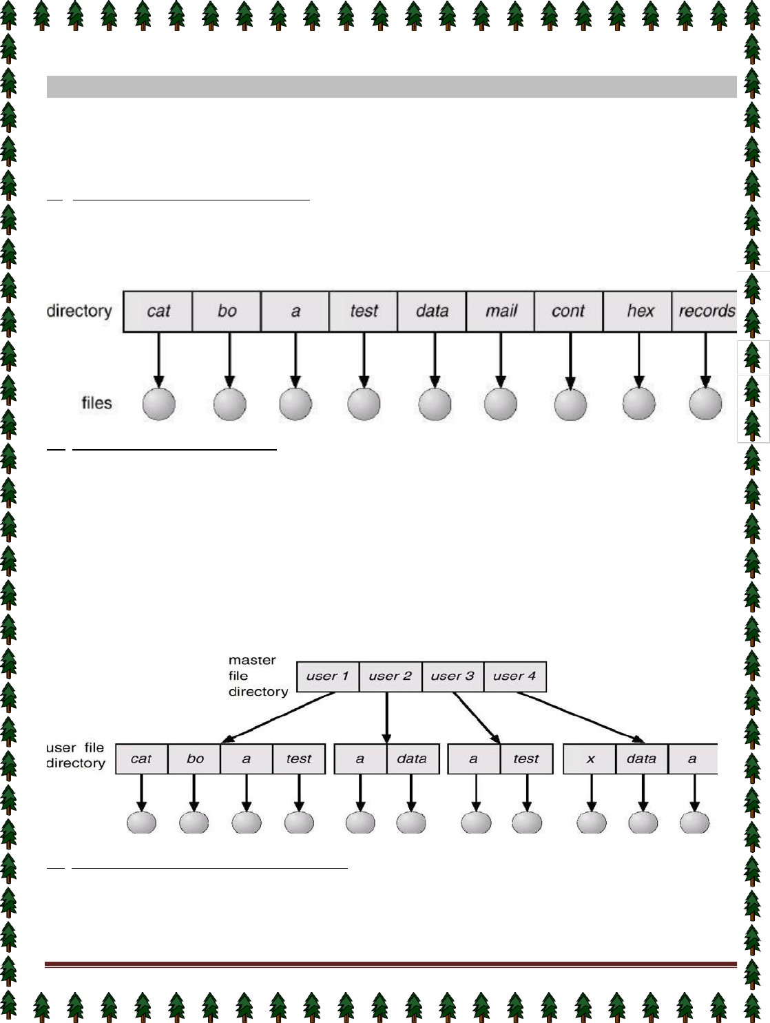
Page 76
modified to include the block number as a parameter. Thus, we have read n, where n is the
block number, rather than read next, and write n rather than write next.
DIRECTORY STRUCTURE
A directory is an object that contains the names of file system objects. File system
allows the users to organize files and other file system objects through the use of directories.
The structure created by placement of names in directories can take a number of forms: Single-
level tree, Two-level tree, multi-level tree or cyclic graph.
1. Single-Level Directory: The simplest directory structure is the single-level
directory. All files are contained in the same directory, which is easy to support and
understand. A single-level directory has significant limitations, when the number of files
increases or when the system has more than one user. Since all files are in the same directory,
they must have unique names.
2. Two-Level Directory: In the two-level directory structure, each user has its own
user file directory (UFD). Each UFD has a similar structure, but lists only the files of a single
user. When a user job starts or a user logs in, the system's master file directory (MFD) is
searched. The MFD is indexed by user name or account number, and each entry points to the
UFD for that user.
When a user refers to a particular file, only his own UFD is searched. Different users
may have files with the same name, as long as all the file names within each UFD are unique.
To create a file for a user, the operating system searches only that user's UFD to
ascertain whether another file of that name exists. To delete a file, the operating system
confines its search to the local UFD; thus, it cannot accidentally delete another user's file that
has the same name.
3. Tree-structured directories: A tree structure is A more powerful and flexible
approach to organize files and directories in hierarchical. There is a master directory, which
has under it a number of user directories. Each of these user directories may have sub-
directories and files as entries. This is true at any level: That is, at any level, a directory may
consist of entries for subdirectories and/or entries for files.
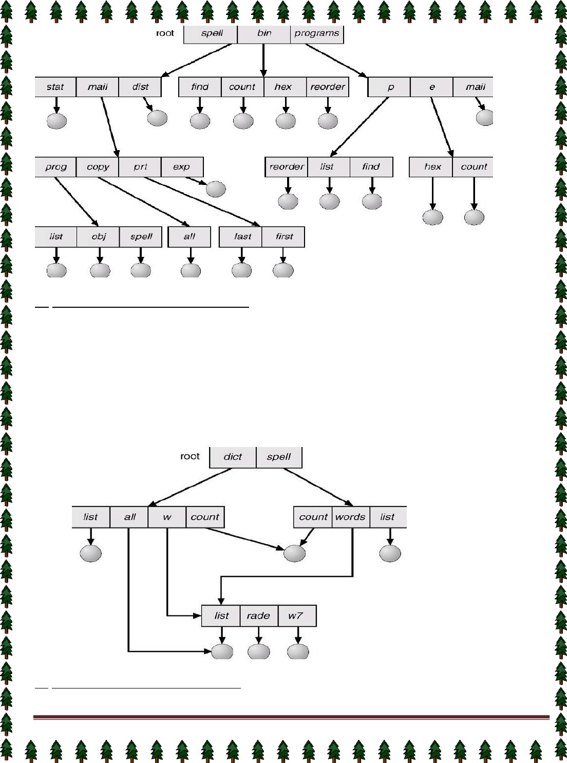
Page 77
4. Acyclic-Graph Directories:
An
acyclic graph
allows directories to have shared subdirectories and files. The
same
file or subdirectory may be in two different directories. An acyclic graph is a natural
generalization of the tree structured directory scheme.
A shared file (or directory) is not the same as two copies of the file. With two copies,
each programmer can view the copy rather than the original, but if one programmer changes
the file, the changes will not appear in the other's copy.
Shared files and subdirectories can be implemented in several ways. A common way is
to create a new directory entry called a link. A link is a pointer to another file or subdirectory.
5. General Graph Directory:
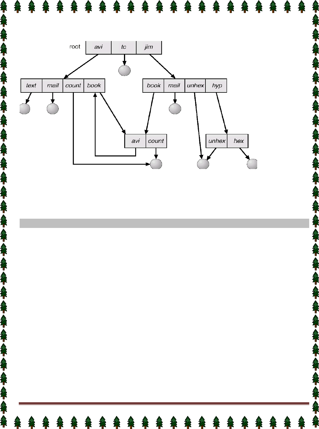
Page 78
When we add links to an existing tree-structured directory, the tree structure is
destroyed, resulting in a simple graph structure.
SECONDARY STORAGE STRUCTURE
DISKS STRUCTURE
Magnetic disks provide the bulk of secondary storage for modern computer systems.
Each disk
platter
has a flat circular shape, like a CD. Common platter diameters range from
1.8 to 5.25 inches. The two surfaces of a platter are covered with a magnetic material. We store
information by recording it magnetically on the platters.
A read-write head "flies" just above each surface of every platter. The heads are
attached to a disk arm, which moves all the heads as a unit. The surface of a platter is
logically divided into circular tracks, which are subdivided into sectors. The set of tracks that
are at one arm position forms a cylinder. There may be thousands of concentric cylinders in a
disk drive, and each track may contain hundreds of sectors. The storage capacity of common
disk drives is measured in gigabytes.
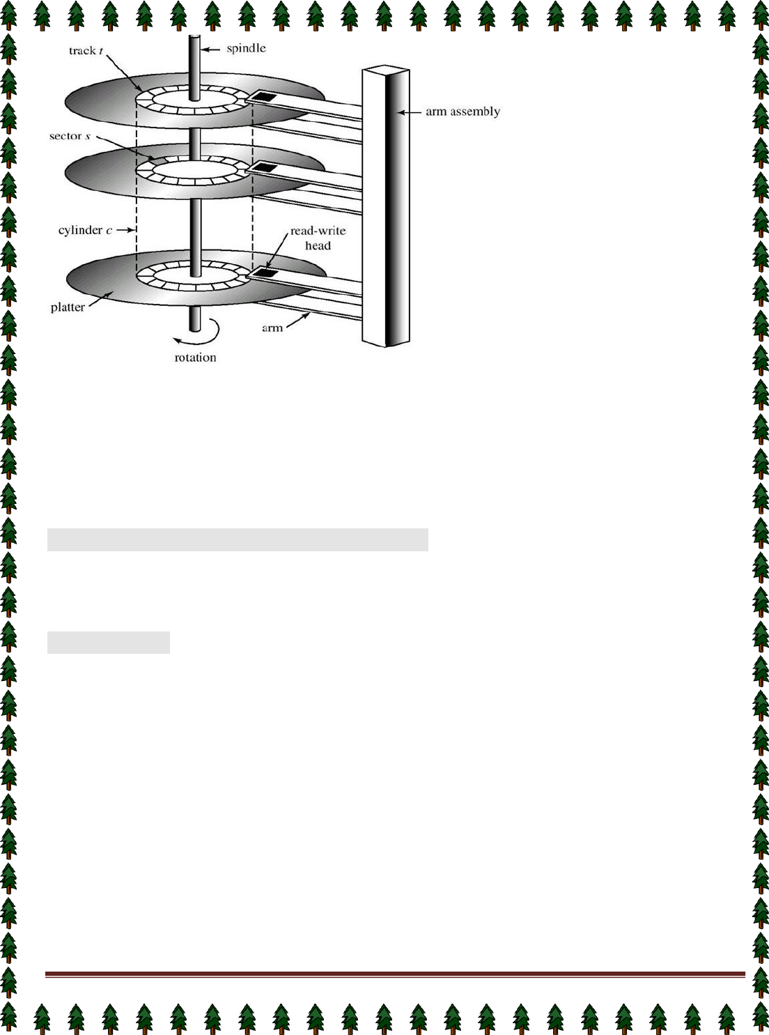
Page 79
(Structure of Magnetic disks (Harddisk drive))
When the disk is in use, a drive motor spins it at high speed. Most drives rotate 60 to
200 times per second. Disk speed has two parts. The
transfer rate
is the rate at which data
flow between the drive and the computer. The
positioning time (or random-access time)
consists of
seek time
and
rotational latency
. The
seek time is
the time to move the disk arm
to the desired cylinder. And the
rotational latency is
the time for the desired sector to rotate
to the disk head
.
Typical disks can transfer several megabytes of data per second and they
have seek times and rotational latencies of several milliseconds.
Capacity of Magnetic disks(C) = S x T x P x N
Where S= no. of surfaces = 2 x no. of disks, T= no. of tracks in a surface,
P= no. of sectors per track, N= size of each sector
Transfer Time: The transfer time to or from the disk depends on the rotation speed of the
disk in the following fashion:
T = b
/
( r x N)
Where
T
= transfer time, b=number of bytes to be transferred,
N
= number of bytes on a track,
r= rotation speed, in revolutions per second.
Modern disk drives are addressed as large one-dimensional arrays of
logical blocks,
where the logical block is the smallest unit of transfer. The one-dimensional array of logical
blocks is mapped onto the sectors of the disk sequentially. Sector 0 is the first sector of the
first track on the outermost cylinder. The mapping proceeds in order through that track, then
through the rest of the tracks in that cylinder, and then through the rest of the cylinders from
outermost to innermost.
By using this mapping, we can convert a logical block number into an old-style disk
address that consists of a cylinder number, a track number within that cylinder, and a sector
number within that track. In practical, it is difficult to perform this translation, for two
reasons. First, most disks have some defective sectors, but the mapping hides this by
substituting spare sectors from elsewhere on the disk. Second, the number of sectors per track
is not a constant on some drives.
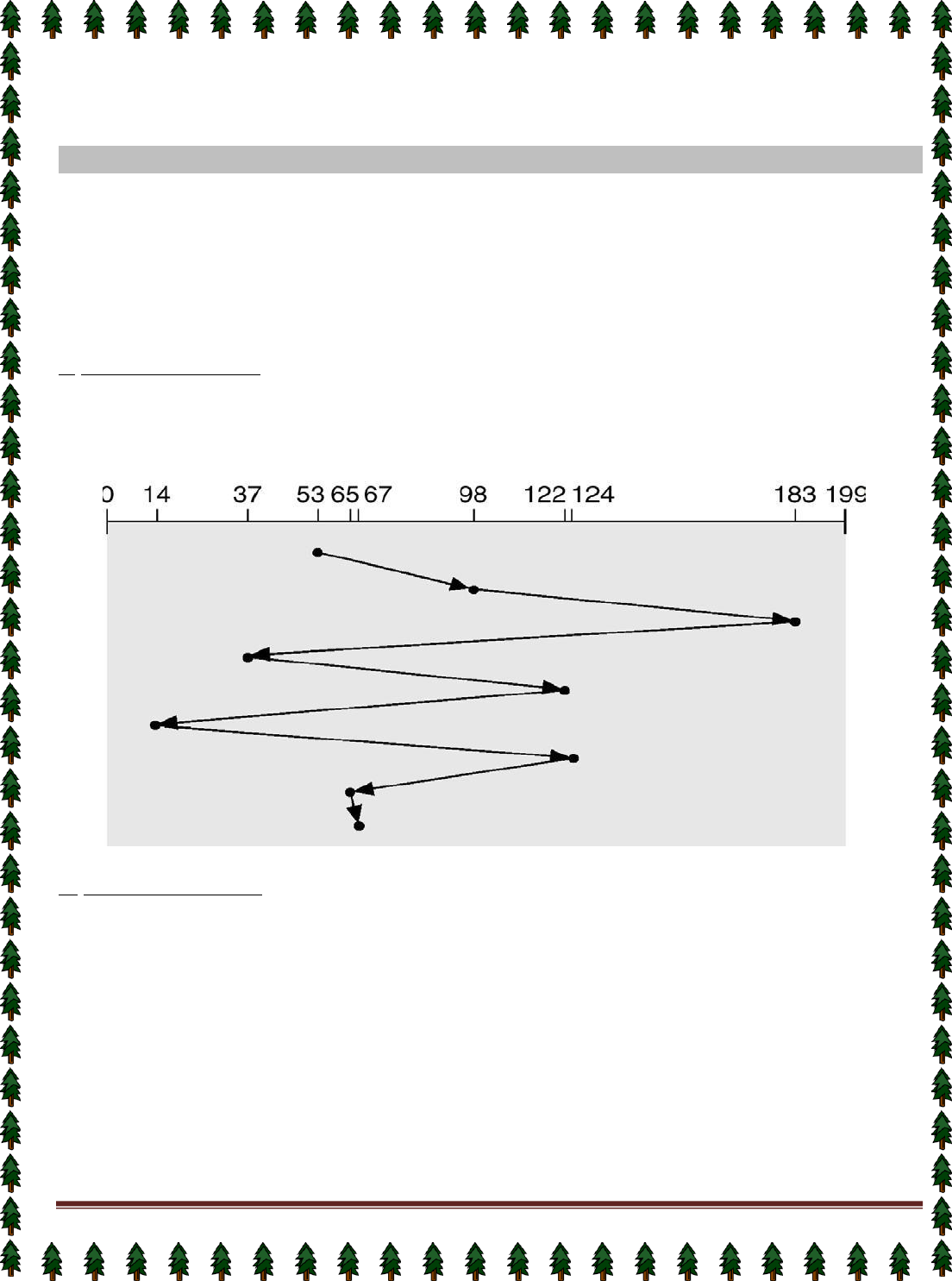
Page 80
The density of bits per track is uniform. This is called Constant linear velocity (CLV).
The disk rotation speed can stay constant and the density of bits decreases from inner tracks
to outer tracks to keep the data rate constant. This method is used in hard disks and is known
as constant angular velocity (CAV).
DISK SCHEDULING
The seek time is the time for the disk arm to move the heads to the cylinder containing
the desired sector. The rotational latency is the time waiting for the disk to rotate the desired
sector to the disk head. The disk bandwidth is the total number of bytes transferred divided
by the total time between the first request for service and the completion of the last transfer.
We can improve both the access time and the bandwidth by scheduling the servicing of
disk I/O requests in a good order. Several algorithms exist to schedule the servicing of disk
I/O requests as follows:
1.
FCFS Scheduling
The simplest form of scheduling is first-in-first-out (FIFO) scheduling, which processes
items from the queue in sequential order. We illustrate this with a request queue (0-199):
98, 183, 37, 122, 14, 124, 65, 67
Consider now the Head pointer is in cylinder 53.
(FCFS disk scheduling)
2.
SSTF Scheduling
It stands for shortest-seek-time-first (SSTF) algorithm. The SSTF algorithm selects the
request with the minimum seek time from the current head position. Since seek time increases
with the number of cylinders traversed by the head, SSTF chooses the pending request closest
to the current head position. We illustrate this with a request queue (0-199):
98, 183, 37, 122, 14, 124, 65, 67
Consider now the Head pointer is in cylinder 53.
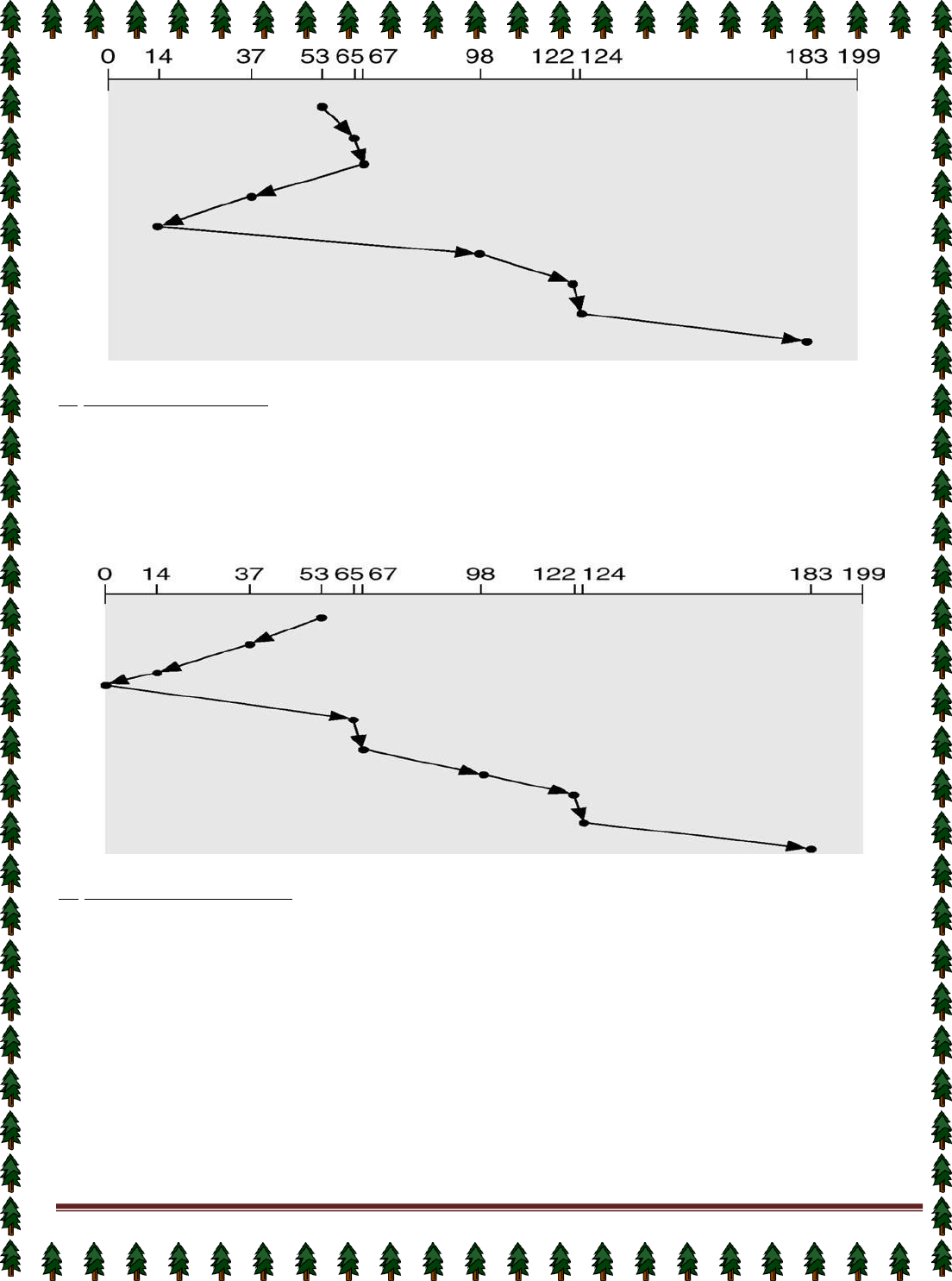
Page 81
(SSTF disk scheduling)
3.
SCAN Scheduling
In the SCAN algorithm, the disk arm starts at one end of the disk, and moves toward
the other end, servicing requests as it reaches each cylinder, until it gets to the other end of the
disk. At the other end, the direction of head movement is reversed, and servicing continues.
The head continuously scans back and forth across the disk. We illustrate this with a request
queue (0-199): 98, 183, 37, 122, 14, 124, 65, 67
Consider now the Head pointer is in cylinder 53.
(SCAN disk scheduling)
4.
C-SCAN Scheduling
Circular
SCAN (C-SCAN)
scheduling is a variant of SCAN designed to provide a
more uniform wait time. Like SCAN, C-SCAN moves the head from one end of the disk to the
other, servicing requests along the way. When the head reaches the other end, it immediately
returns to the beginning of the disk, without servicing any requests on the return trip. The C-
SCAN scheduling algorithm essentially treats the cylinders as a circular list that wraps
around from the final cylinder to the first one. We illustrate this with a request queue (0-199):
98, 183, 37, 122, 14, 124, 65, 67. Consider now the Head pointer is in cylinder 53.
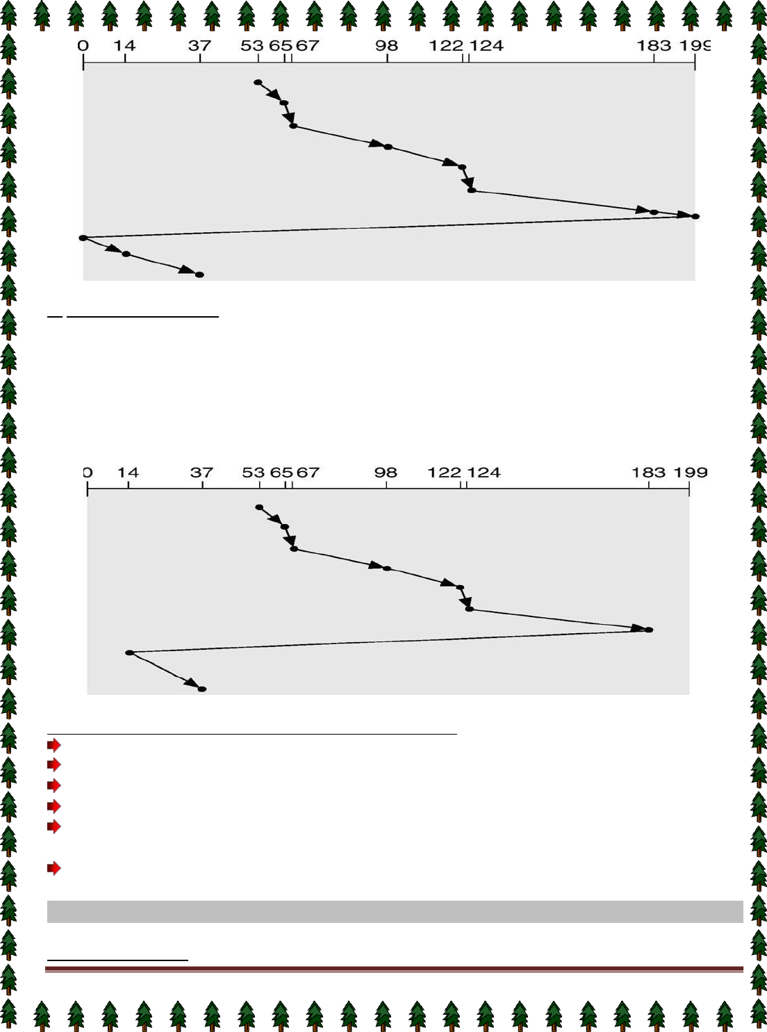
Page 82
(C-SCAN disk scheduling)
5.
LOOK Scheduling
Practically, both SCAN and C-SCAN algorithm is not implemented this way. More
commonly, the arm goes only as far as the final request in each direction. Then, it reverses
direction immediately, without going all the way to the end of the disk. These versions of
SCAN and C-SCAN are called
LOOK
and
C-LOOK
scheduling, because they look for a
request before continuing to move in a given direction. We illustrate this with a request queue
(0-199): 98, 183, 37, 122, 14, 124, 65, 67
Consider now the Head pointer is in cylinder 53.
(C-LOOK disk scheduling)
Selection of a Disk-Scheduling Algorithm
SSTF is common and has a natural appeal.
SCAN and C-SCAN perform better for systems that place a heavy load on the disk.
Performance depends on the number and types of requests.
Requests for disk service can be influenced by the file allocation method.
The disk-scheduling algorithm should be written as a separate module of the operating
system, allowing it to be replaced with a different algorithm if necessary.
Either SSTF or LOOK is a reasonable choice for the default algorithm.
DISK MANAGEMENT
The operating system is responsible for several aspects of disk management.
Disk Formatting

Page 83
A new magnetic disk is a blank slate. It is just platters of a magnetic recording material.
Before a disk can store data, it must be divided into sectors that the disk controller can read
and write. This process is called low-level formatting (or physical formatting).
Low-level formatting
fills the disk with a special data structure for each sector. The
data structure for a sector consists of a header, a data area, and a trailer. The header and
trailer contain information used by the disk controller, such as a sector number and an
error-
correcting code (ECC).
To use a disk to hold files, the operating system still needs to record its own data
structures on the disk. It does so in two steps. The first step is to
partition
the disk into one or
more groups of cylinders. The operating system can treat each partition as though it were a
separate disk. For instance, one partition can hold a copy of the operating system's executable
code, while another holds user files. After partitioning, the second step is
logical formatting
(or creation of a file system). In this step, the operating system stores the initial file-system
data structures onto the disk.
Boot Block
When a computer is powered up or rebooted, it needs to have an initial program to
run. This initial program is called bootstrap program. It initializes all aspects of the system
(i.e. from CPU registers to device controllers and the contents of main memory) and then
starts the operating system.
To do its job, the bootstrap program finds the operating system kernel on disk, loads
that kernel into memory, and jumps to an initial address to begin the operating-system
execution.
For most computers, the bootstrap is stored in read-only memory
(ROM).
This location
is convenient, because ROM needs no initialization and is at a fixed location that the
processor can start executing when powered up or reset. And since ROM is read only, it
cannot be infected by a computer virus. The problem is that changing this bootstrap code
requires changing the ROM hardware chips.
For this reason, most systems store a tiny bootstrap loader program in the boot ROM,
whose only job is to bring in a full bootstrap program from disk. The full bootstrap program
can be changed easily: A new version is simply written onto the disk. The full bootstrap
program is stored in a partition (at a fixed location on the disk) is called the boot blocks. A
disk that has a boot partition is called a boot disk or system disk.
Bad Blocks
Since disks have moving parts and small tolerances, they are prone to failure.
Sometimes the failure is complete, and the disk needs to be replaced, and its contents restored
from backup media to the new disk.
More frequently, one or more sectors become defective. Most disks even come from the
factory with bad blocks. Depending on the disk and controller in use, these blocks are
handled in a variety of ways.
The controller maintains a list of bad blocks on the disk. The list is initialized during
the low-level format at the factory, and is updated over the life of the disk. The controller can
be told to replace each bad sector logically with one of the spare sectors. This scheme is
known as sector sparing or forwarding.
SWAP-SPACE MANAGEMENT

Page 84
The swap-space management
is a low-level task of the operating system. The main
goal for the design and implementation of swap space is to provide the best throughput for
the virtual-memory system.
Swap-Space Use
Swap space is used in various ways by different operating systems depending on the
implemented memory-management algorithms.
Those systems are implemented swapping, they may use swap space to hold the entire
process image, including the code and data segments. The amount of swap space needed on a
system can vary depending on the amount of physical memory,
Swap-Space Location
A
swap space can reside in two places: Swap space can be carved out of the normal file
system, or it can be in a separate disk partition.
If the swap space is simply a large file within the file system, normal file-system
routines can be used to create it, name it, and allocate its space. This approach is easy to
implement and is also inefficient.
Alternatively, swap space can be created in a separate disk partition. No file system or
directory structure is placed on this space. A separate swap-space storage manager is used to
allocate and deallocate the blocks. This manager uses algorithms optimized for speed and
storage efficiency.
RAID STRUCTURE
A Redundant Array of Inexpensive Disks(RAID) may be used to increase disk reliability.
RAID may be implemented in hardware or in the operating system.
The RAID consists of seven levels, zero through six. These levels designate different
design architectures that share three common characteristics:
RAID is a set of physical disk drives viewed by the operating system as a single logical
drive.
Data are distributed across the physical drives of an array in a scheme known as striping,
described subsequently.
Redundant disk capacity is used to store parity information, which guarantees data
recoverability in case of a disk failure.
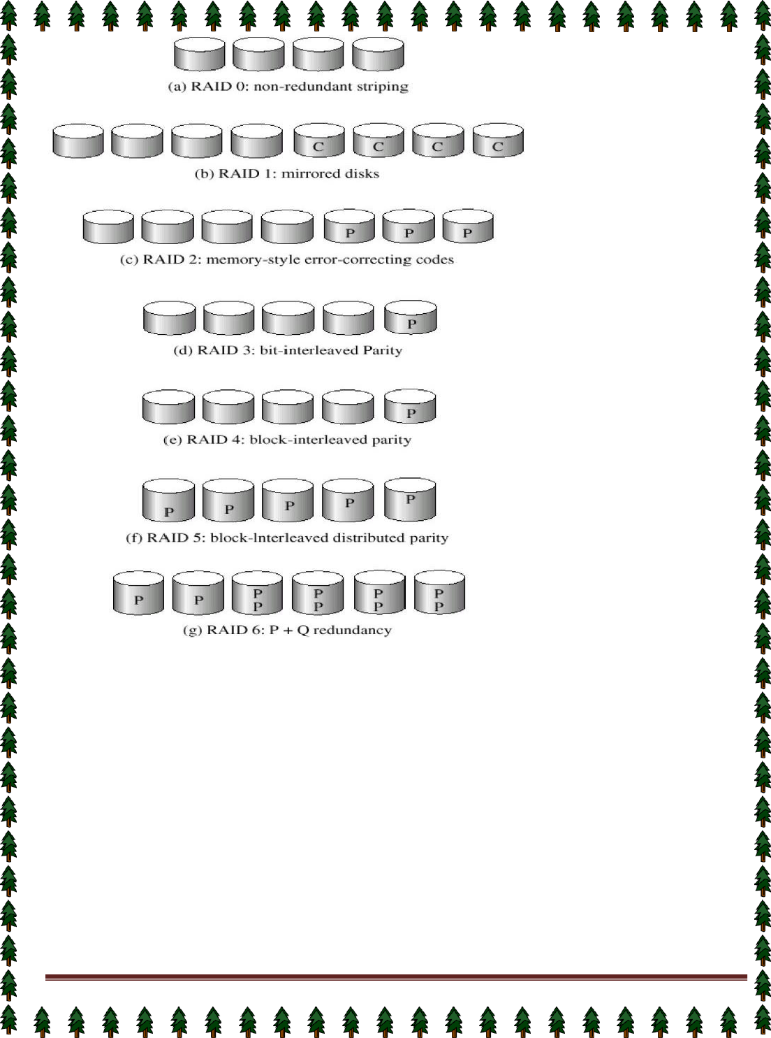
Page 85
(RAID
levels)
(Here P indicates error-correcting bits and C indicates a second copy of the data)
The RAID levels are described as follows:
RAID Level 0:
RAID level 0 refers to disk arrays with striping at the level of blocks, but
without any redundancy (such as parity bits). Figure(a) shows an array of size 4.
RAID Level 1:
RAID level 1 refers to disk mirroring. Figure (b) shows a mirrored
organization that holds four disks' worth of data.
RAID Level 2: RAID level 2 is also known as memory-style error-correcting code (ECC)
organization. Each byte in a memory system may have a parity bit associated with it that
records whether the numbers of bits in the byte set to 1 is even (parity=O) or odd
(parity=l). The idea of ECC can be used directly in disk arrays via striping of bytes across
disks.
RAID level 3: RAID level 3, or bit-interleaved parity organization, improves on level 2 by
noting that, disk controllers can detect whether a sector has been read correctly, so a single
parity bit can be used for error correction, as well as for detection. The idea is as follows. If
one of the sectors gets damaged, we know exactly which sector it is, and, for each bit in the

Page 86
sector, we can figure out whether it is a 1 or a 0 by computing the parity of the
corresponding bits from sectors in the other disks. If the parity of the remaining bits is
equal to the stored parity, the missing bit is 0; otherwise, it is 1.
RAID Level 4: RAID level 4 or block-interleaved parity organization uses block-level
striping, as in RAID 0 and in addition keeps a parity block on a separate disk for
corresponding blocks from N other disks. This scheme is shown pictorially in Figure(e). If
one of the disks fails, the parity block can be used with the corresponding blocks from the
other disks to restore the blocks of the failed disk.
RAID level 5: RAID level 5 or block-interleaved distributed parity is similar as level 4
but level 5 spreading data and parity among all N + 1 disks, rather than storing data in N
disks and parity in one disk. For each block, one of the disks stores the parity, and the
others store data. By spreading the parity across all the disks in the set, RAID 5 avoids the
potential overuse of a single parity disk that can occur with RAID 4.
RAID Level 6: RAID level 6 (is also called the P+Q redundancy scheme) is much like
RAID level 5, but stores extra redundant information to guard against multiple disk
failures. Instead of using parity, error-correcting codes such as the Reed-Solomon codes
are used.
I/O SYSTEM
The role of the operating system in computer I/O is to manage and control I/O
operations and I/O devices. A device communicates with a computer system by sending
signals over a cable or even through the air. The device communicates with the machine via a
connection point. If one or more devices use a common set of wires for communication, the
connection is called
a bus.
When device A has a cable that plugs into device B, and device B has a cable that plugs
into device C, and device C plugs into a port on the computer, this arrangement is called a
daisy chain. A daisy chain usually operates as a bus.
Buses are used widely in computer architecture as follows:
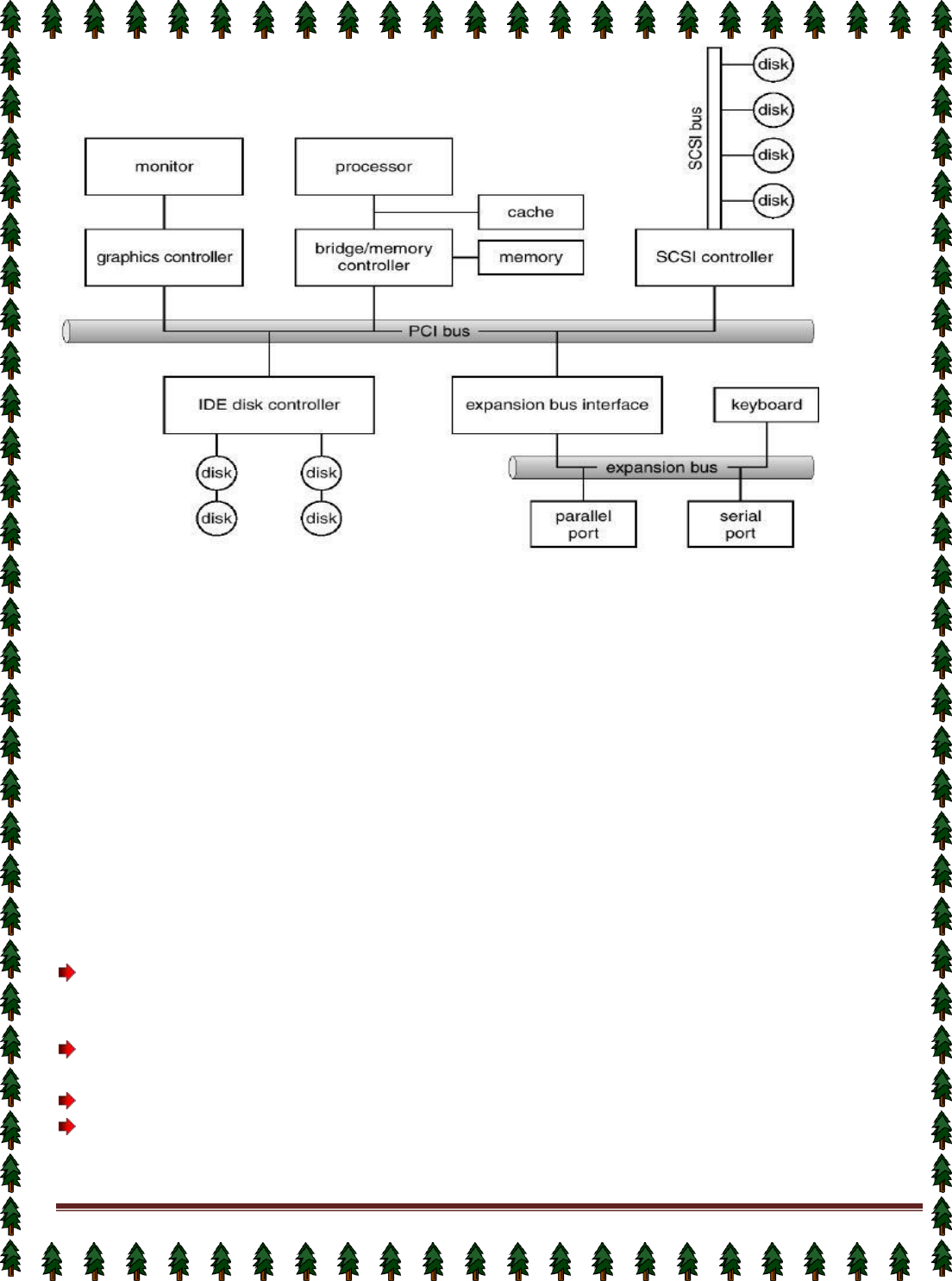
Page 87
(A typical PC bus structure)
This figure shows a
PC1
bus (the common PC system bus) that connects the processor-
memory subsystem to the fast devices, and an expansion bus that connects relatively slow
devices such as the keyboard and serial and parallel ports. In the upper-right portion of the
figure, four disks are connected together on a SCSI bus plugged into a SCSI controller.
A controller is a collection of electronics that can operate a port, a bus, or a device. A
serial-port controller is a simple device controller. It is a single chip (or portion of a chip) in
the computer that controls the signals on the wires of a serial port.
Since the SCSI protocol is complex, the SCSI bus controller is often implemented as a
separate circuit board (or a host adapter) that plugs into the computer. It contains a processor,
microcode, and some private memory to enable it to process the SCSI protocol messages.
Some devices have their own built-in controllers. This board is the disk controller. It
has microcode and a processor to do many tasks, such as bad-sector mapping, prefetching,
buffering, and caching.
A
n
I
/
O
p
o
r
t
co
nsi
sts
o
f
f
o
u
r
r
e
gi
ste
r
s,
ca
ll
e
d
t
h
e
s
ta
tu
s
,
c
o
n
tr
o
l,
d
ata
-
in
,
a
nd d
ata
-
ou
t
registers.
The status register contains bits that can be read by the host. These bits indicate states such
as whether the current command has completed, whether a byte is available to be read
from the data-in register, and whether there has been a device error.
The control register can be written by the host to start a command or to change the mode
of a device.
The data-in register is read by the host to get input.
The data-out register is written by the host to send output.
The external devices can be grouped into three categories:

Page 88
1.
Human readable:
Suitable for communicating with the computer user. Examples include
printers and terminals, the latter consisting of video display, keyboard, and perhaps other
devices such as a mouse.
2.
Machine readable:
Suitable for communicating with electronic equipment. Examples are
disk drives, USB keys, sensors, controllers, and actuators.
3.
Communication:
Suitable for communicating with remote devices. Examples are digital
line drivers and modems.
ORGANIZATION OF THE I/O FUNCTION(I/O Technique)
There are three techniques for performing I/O operations:
1.
Programmed I/O: The processor issues an I/O command, on behalf of a process, to an
I/O module; that process busy waits for the operation to be completed before proceeding.
2.
Interrupt-driven I/O: The processor issues an I/O command on behalf of a process.
There are two possibilities. If the I/O instruction from the process is non blocking, then
the processor continues to execute instructions from the process that issued the I/O
command. If the I/O instruction is blocking, then the next instruction that the processor
executes is from the OS, which will put the current process in a blocked state and schedule
another process.
3.
Direct memory access (DMA): A DMA module controls the exchange of data between
main memory and an I/O module. The processor sends a request for the transfer of a
block of data to the DMA module and is interrupted only after the entire block has been
transferred.
Interrupt-driven I/O
The basic interrupt mechanism works as follows.
The CPU hardware has a wire called the interrupt-request line that the CPU senses after
executing every instruction.
When the CPU detects that a controller has asserted a signal on the interrupt request line,
the CPU saves a small amount of state, such as the current value of the instruction pointer,
and jumps to the interrupt-handler routine at a fixed address in memory.
The interrupt handler determines the cause of the interrupt, performs the necessary
processing, and executes a return from interrupt instruction to return the CPU to the
execution state prior to the interrupt.
The above mechanism concludes that the device controller
raises
an interrupt by asserting
a signal on the interrupt request line, the CPU
catches
the interrupt and
dispatches
to the
interrupt handler, and the handler
clears
the interrupt by servicing the device.
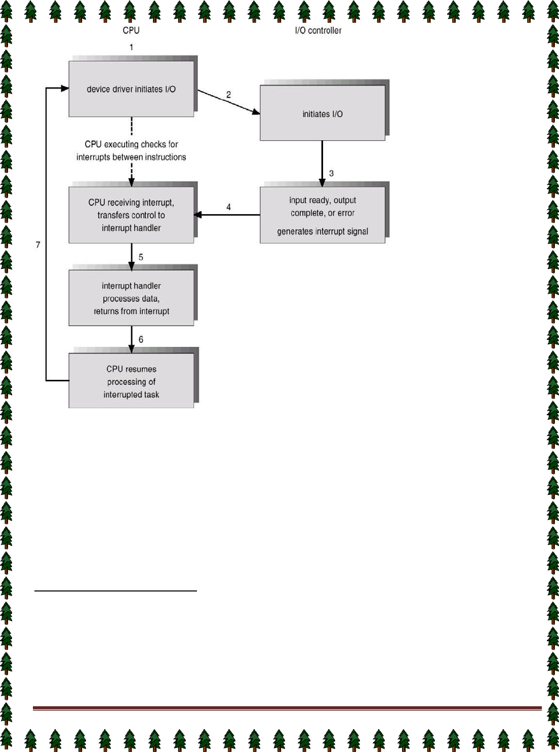
Page 89
(
Diagram of Interrupt-driven I/O cycle)
In a modern operating system, we need more sophisticated interrupt-handling features as
follows:
First, we need the ability to defer interrupt handling during critical processing.
Second, we need an efficient way to dispatch to the proper interrupt handler for a device.
Third, we need multilevel interrupts, so that the operating system can distinguish between
high- and low-priority interrupts, and can respond with the appropriate degree of
urgency.
In modern computer hardware, these three features are provided by the CPU and by
the interrupt-controller hardware.
Direct Memory Access
The DMA unit is capable of mimicking the processor and of taking over control of the
system bus just like a processor. It needs to do this to transfer data to and from memory over
the system bus. The DMA technique works as follows:
When the processor wishes to read or write a block of data, it issues a command to the
DMA module by sending to the DMA module the following information:
Whether a read or write is requested, using the read or write control line
between the processor and the DMA module.
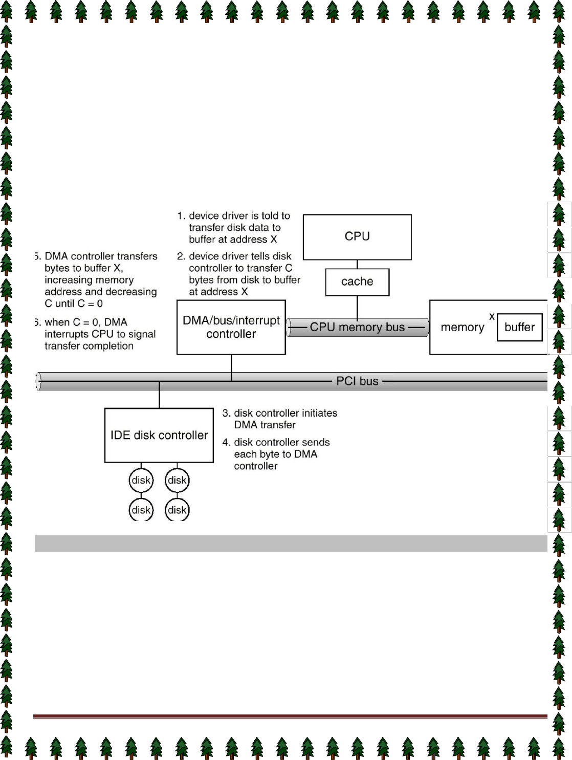
Page 90
The address of the I/O device involved, communicated on the data lines.
The starting location in memory to read from or write to, communicated on the
data lines and stored by the DMA module in its address register.
The number of words to be read or written, again communicated via the data
lines and stored in the data count register.
Then the processor continues with other work. It has delegated this I/O operation to the
DMA module.
The DMA module transfers the entire block of data, one word at a time, directly to or from
memory, without going through the processor.
When the transfer is complete, the DMA module sends an interrupt signal to the
processor. Thus, the processor is involved only at the beginning and end of the transfer.
(Steps in a DMA transfer)
APPLICATION I/O INTERFACE
I/O system calls encapsulate device behaviors in generic classes. Each general kind is
accessed through a standardized set of functions, called an interface. The differences are
encapsulated in kernel modules called device drivers that internally are custom tailored to
each device, but that export one of the standard interfaces.
Devices vary in many dimensions:
o
Character-stream or block
o
Sequential or random-access
o
Sharable or dedicated
o
Speed of operation
o
read-write, read only, or write only
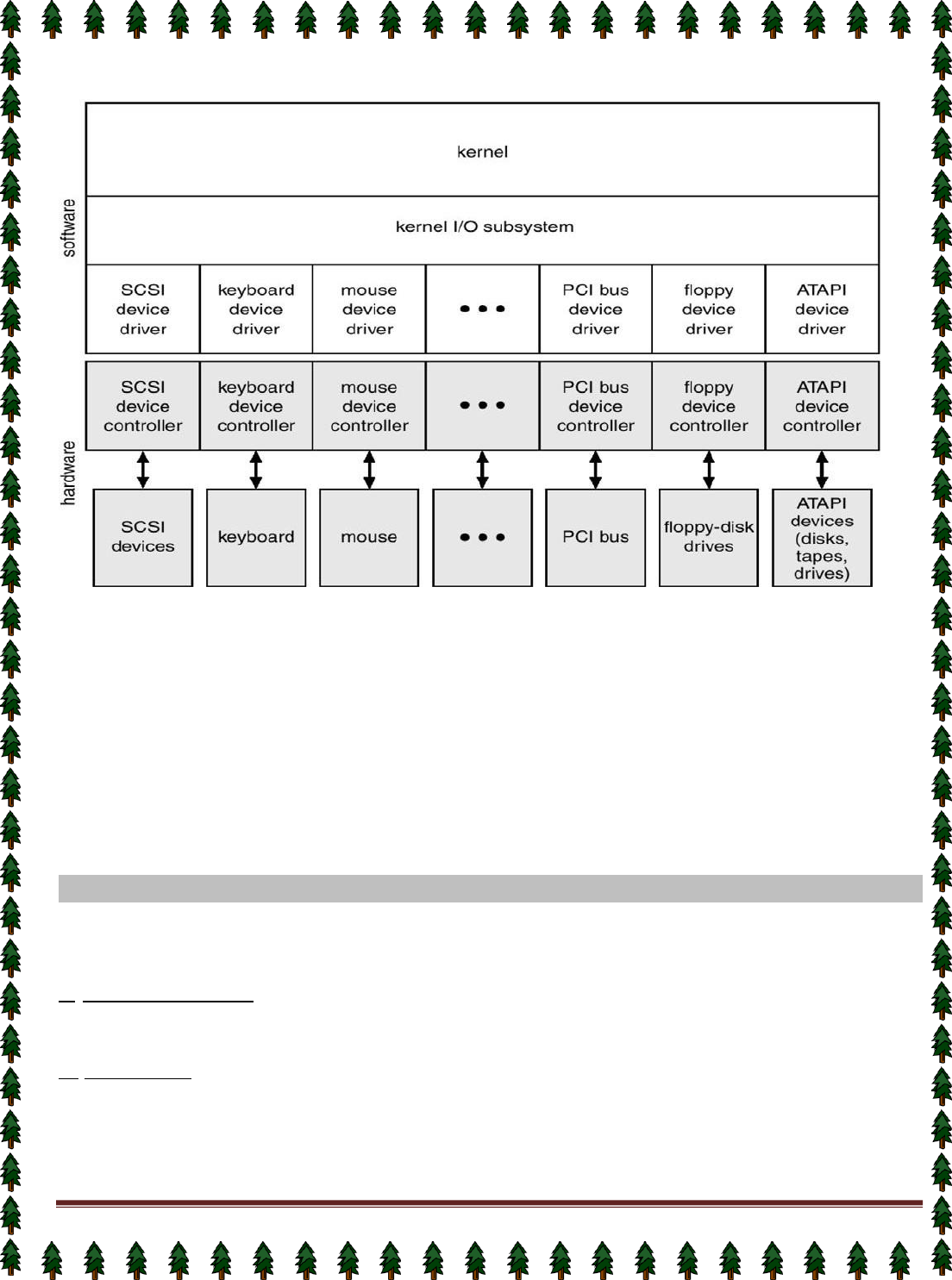
Page 91
(Diagram of a kernel I/O structure)
The purpose of the device-driver layer is to hide the differences among device
controllers from the I/O subsystem of the kernel, much as the I/O system calls encapsulate
the behavior of devices in a few generic classes that hide hardware differences from
applications. Making the I/O subsystem independent of the hardware simplifies the job of the
operating-system developer. It also benefits the hardware manufacturers. They either design
new devices to be compatible with an existing host controller interface (such as SCSI-2), or
they write device drivers to interface the new hardware to popular operating systems. Thus,
new peripherals can be attached to a computer without waiting for the operating-system
vendor to develop support code.
KERNEL I/O SUBSYSTEM
Kernels provide many services related to I/O. Several services (i.e. scheduling,
buffering, caching, spooling, device reservation and error handling) are provided by the
kernel's I/O subsystem and build on the hardware and device driver infrastructure.
1.
I/O Scheduling: It is used to schedule a set of I/O requests that means to determine a
good order in which to execute them. Scheduling can improve overall system performance
and can reduce the average waiting time for I/O to complete.
2.
Buffering:
A
buffer
is a memory area that stores data while they are transferred between
two devices or between a device and an application. Buffering is done for three reasons.
One reason is to cope with a speed mismatch between the producer and consumer of a
data stream.

Page 92
A second use of buffering is to adapt between devices that have different data-transfer
sizes.
A third use of buffering is to support copy semantics for application I/O.
3.
Caching:
A
cache
is a region of fast memory that holds copies of data. Access to the
cached copy is more efficient than access to the original. Cache is used to improve the I/O
efficiency for files that are shared by applications or that are being written and reread rapidly.
The difference between a buffer and a cache is that a buffer may hold the only existing
copy of a data item, whereas a cache just holds a copy on faster storage of an item that resides
elsewhere. Caching and buffering are distinct functions, but sometimes a region of memory
can be used for both purposes.
4.
Spooling:
A
spool
is a buffer that holds output for a device, such as a printer, that cannot
accept interleaved data streams. Although a printer can serve only one job at a time, several
applications may wish to print their output concurrently, without having their output mixed
together. The operating system solves this problem by intercepting all output to the printer.
Each application's output is spooled to a separate disk file. When an application
finishes printing, the spooling system queues the corresponding spool file for output to the
printer.
The spooling system copies the queued spool files to the printer one at a time. The
operating system provides a control interface that enables users and system administrators to
display the queue, to remove unwanted jobs before those jobs print, to suspend printing
while the printer is serviced, and so on.
5.
Device Reservation:
It provides support for exclusive device access, by enabling a process to allocate an idle
device, and to deallocate that device when it is no longer needed. Many operating systems
provide functions that enable processes to coordinate exclusive access among them. It
watches out for deadlock to avoid.
Transforming I/O request to Hardware Operations
Consider reading a file from disk for a process:
Determine device holding file
Translate name to device representation
Physically read data from disk into buffer
Make data available to requesting process
Return control to process
The following steps are described the lifecycle of a blocking read request:
1.
A process issues a blocking
read()
system call to a file descriptor of a file that has been
opened previously.
2.
The system-call code in the kernel checks the parameters for correctness. In the case of
input, if the data are already available in the buffer cache, the data are returned to the
process and the I/O request is completed.
3.
Otherwise, a physical I/O needs to be performed, so the process is removed from the run
queue and is placed on the wait queue for the device, and the I/O request is scheduled.
Eventually, the I/O subsystem sends the request to the device driver. Depending on the
operating system, the request is sent via a subroutine call or via an in-kernel message.
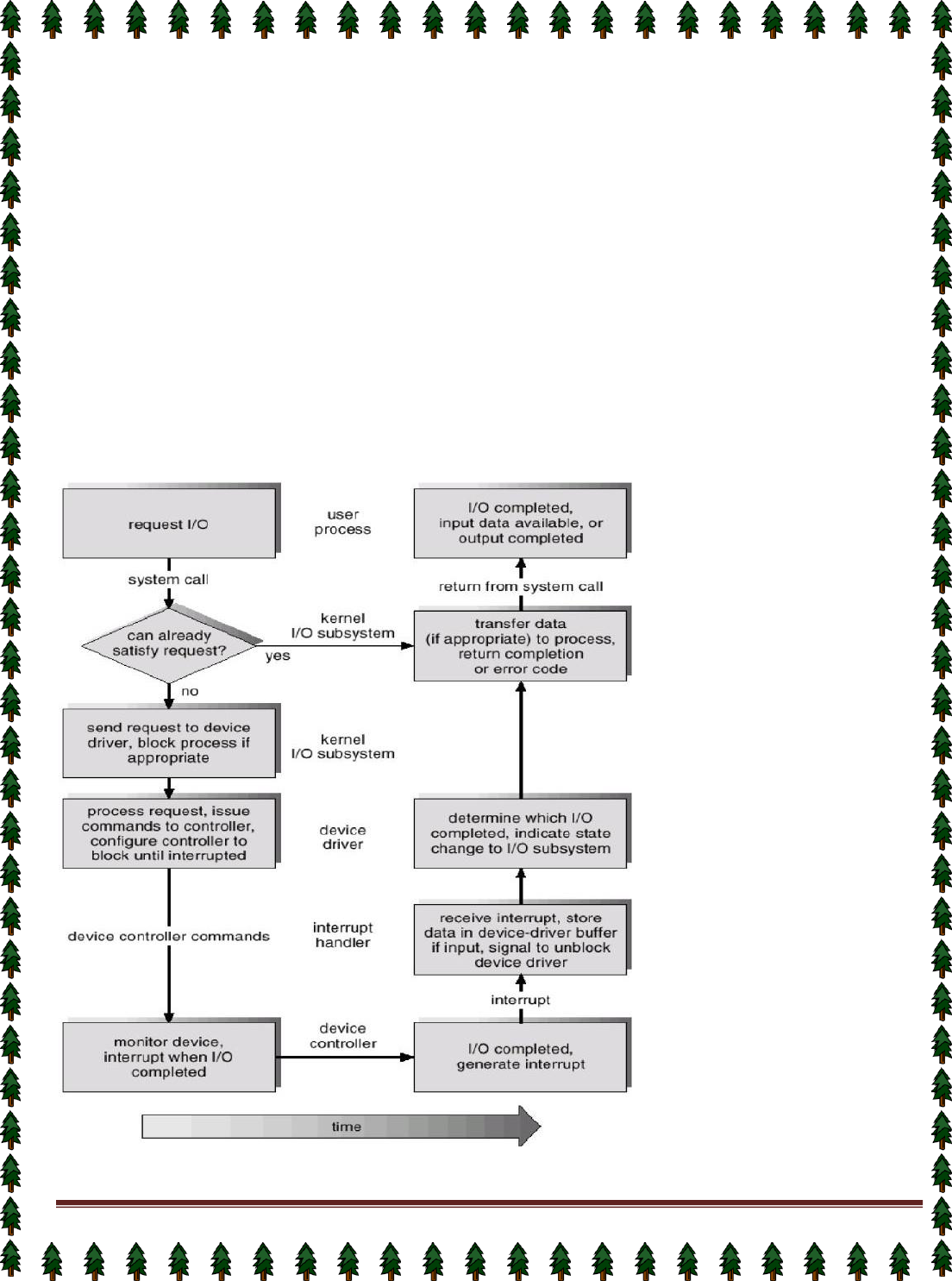
Page 93
4.
The device driver allocates kernel buffer space to receive the data, and schedules the I/O.
Eventually, the driver sends commands to the device controller by writing into the device
control registers.
5.
The device controller operates the device hardware to perform the data transfer.
6.
The driver may poll for status and data, or it may have set up a DMA transfer into kernel
memory. We assume that the transfer is managed by a DMA controller, which generates
an interrupt when the transfer completes.
7.
The correct interrupt handler receives the interrupt via the interrupt-vector table, stores
any necessary data, signals the device driver, and returns from the interrupt.
8.
The device driver receives the signal, determines which I/O request completed,
determines the request's status, and signals the kernel I/O subsystem that the request has
been completed.
9.
The kernel transfers data or returns codes to the address space of the requesting process,
and moves the process from the wait queue back to the ready queue.
10.
Moving the process to the ready queue unblocks the process. When the scheduler assigns
the process to the CPU, the process resumes execution at the completion of the system call.
(The life cycle of an I/O request)
